http://dx.doi.org/10.4236/am.2013.412218
A Forward-Looking Nash Game and Its Application to
Achieving Pareto-Efficient Optimization
Jie Ren1, Kai-Kit Wong2, Jianjun Hou1
1School of Electronics and Information Engineering, Beijing Jiaotong University, Beijing, China 2Department of Electronic and Electrical Engineering, University College London,
Torrington Place, London, UK
Email: [email protected], [email protected], [email protected] Received September 19, 2013; revised October 19, 2013; accepted October 26, 2013
Copyright © 2013 Jie Ren et al. This is an open access article distributed under the Creative Commons Attribution License, which permits unrestricted use, distribution, and reproduction in any medium, provided the original work is properly cited.
ABSTRACT
Recognizing the fact that a player’s cognition plays a defining role in the resulting equilibrium of a game of competition, this paper provides the foundation for a Nash game with forward-looking players by presenting a formal definition of the Nash game with consideration of the players’ belief. We use a simple two-firm model to demonstrate its fundamen- tal difference from the standard Nash and Stackelberg games. Then we show that the players’ belief functions can be re- garded as the optimization parameters for directing the game towards a much more desirable equilibrium.
Keywords: Belief; Cognition; Iterative Algorithm; Nash Equilibrium; Pareto-Optimality; Stackelberg
1. Introduction
Game theory has been very well recognized as a branch of applied mathematical tools, best for analyzing the phenomenon of selfish competition, which arises in nu- merous real-life applications ranging from economics to social sciences, and even to engineering problems. Many optimization problems can be viewed as a competition problem.
If there are shared resources, then inherently there will be competition in the allocation of such resources. An individual who participates in the resource allocation always wishes to maximize its payoff. Nevertheless, the player’s return not only depends on its own strategy, but is also dependent on competitors’ responses. As a result, ideally, a player should choose or optimize its strategy based on not only its immediate return but also the possi- ble outcomes of how others might respond to its strategy. Apparently, a player’s cognition (i.e., its belief on how the environment as a whole would react to any of its ac- tion) will be pivotal in the optimization of its strategy for maximizing its payoff and in defining the equilibrium of the game.
In the literature, there are a number of game-theoretic models and they differ in their assumptions on the play- ers’ cognition. Due to this fundamental difference, these models represent different competition environments,
thereby resulting in very different outcomes, which at the steady state are referred to as equilibria. When the com- petition process reaches an equilibrium, by definition, no player would have incentive to change their strategies further to deviate from the equilibrium which is therefore usually considered as a satisfactory outcome to all play- ers.
The most popular model has to be the Nash game [1] in which a player has the belief that other players’ strate- gies are fixed and will not change regardless of what it does. A Nash game is based on such assumption on the players’ cognition. It is noted that the game is still very well defined, although the player’s belief is totally inac- curate.
On the other hand, in a Stackelberg game [2], there is a super player, commonly known as leader, who knows all the information about its competitors, known as follow- ers. In this case, the leader is considered to have perfect cognition and therefore can obtain the most rewarding strategy.
the players. In contrast, the assumption for the Stackel- berg model is too stringent and it is often too difficult to be qualified to be a leader in most practical scenarios. Nevertheless, the Stackelberg equilibrium is highly bene- ficial to the leader. The limitation is that if there were two or more leaders, all of which possess perfect cogni- tion and wish to be the biggest winner, this would lead to a tragedy [3].
In this paper, we recognize the importance of players’ cognition in a game, and focus on how the assumption of the players’ cognition affects the equilibrium. Based on the analysis of Nash and Stackelberg equilibria, we pro- vide a new definition for the Nash game with considera tion of the players’ belief. As a useful byproduct, the new definition facilitates the interpretation of the players’ belief as the optimization parameters, which, if optimized properly, can direct the game towards a Pareto-efficient equilibrium.
2. Preliminaries
2.1. The Two-Firm Model
For illustrative purpose, in this paper, we use a simple two-firm model in economics as an example. In this simple model, there are two firms, Firm A and Firm B. They manufacture an identical product and its unit cost is the same for both firms. In addition, the profit per unit product diminishes as the number of products available in the market increases. In particular, let xa
0 de-note the number of products manufactured by Firm A, and be that manufactured by Firm B. The unit cost is denoted by and the price per product which is set the same by both Firm A and Firm B is assumed to be
a b for some constant . Therefore, the profit functions for Firm A and Firm B are, respectively, given by
0b
x
x
.
c
a x a> 0
, ,
,
a a b a b a
b a b a b b
f x x a x x c x
f x x a x x c x
(1)
In various game-theoretic models, the objective would be for Firm A and Firm B to iteratively optimize their respective strategies, xa and xb, for maximizing their profits (1) in a competitive fashion. Before we examine different equilibria of this two-firm game, we find it useful to first present the general notations of a game.
For a game with K> 1 players, we denote the stra-
tegy profile for player k as k and use
1 2 K
(2)
to represent the strategy profile for all the players.
Moreover, we use to denote a spe-
cific choice of strategy from all the players, where is the strategy adopted by player , and
xk, k
x x
1, , 1, 1, ,
k x xk xk xK
x (3)
denotes the adopted strategy by all the players except player . Likewise, the reward function for player k is denoted by
k
k . If the game converges to an
equilibrium, then we will use the superscript
f x
*
to highlight that the corresponding parameters are at the equilibrium. For instance, we have x* and *
k
f at the equilibrium.
2.2. Nash Competition
Given the competition of K players, if at some point, no one can gain any further by deviating from its present strategy, then the strategy of all the players is said to have reached to an equilibrium [4]. Mathematically, we have
*
and k k: k k k, k .
k x f f x
x x* (4)
Now, proceed to derive the Nash equilibrium for the two-firm example. According to (4), Firm A solves
*
0 , 0 .
max max
a a
a a b a b a
x x
*
f x x a x x c x
(5)
As such, it can be easily shown that
*
* *
d
2 .
d 2
a b
b a a
a
f a x c
a x c x x
x
(6)
Similarly, *
b
x can be derived, resulting the set of
simultaneous equations * *
* *
, 2
. 2
b a
a b
a x c x
a x c x
(7)
As a result, the game governed by (7) will reach the Nash equilibrium
* ,
3 3
ac ac
x , (8)
which leads to the profits
2
2* *, * , . (9)
9 9
a b
a c a c
f f
f
It is worth pointing out here that in Nash equilibrium
when taking d d a
a f
x in the optimization for player A, player A believes that at any given time instance is
optimal and fixed, or b x
*
d 0 d
b
a x
x . This is obviously inaccurate. At the Nash equilibrium in particular, from
k k
x k (1.7), we actually have
*
d
0.5 0
d b
a x
that a Nash player’s cognition and the reality have con-
he profit functi best strategy by According to (10) and using (1
siderable difference and t on
, *
a a b
f x x is in fact only the profit in the ideal situation b b
*
x x
but does not represent the actual profit function due to interaction from player B.
2.3. Stackelberg Competition
A player can benefit more from the rest of the players in cognition about how a game if this player has perfect
others would react to its strategy. This is studied formally by the Stackelberg equilibrium. In the general setting with K players, if player is the leader, it should
know perfectly the response function x
x and therefore is able to obtain the most effective strategy such that
*
: , .
x f f x x
x x (10)
For other players , as they do not have any information about any of the other players’
they can that ot
k
strategies, only assume her players’ strategies are fixed, and will act like a Nash player, see (4). As a result, we have
*
*
and k k: k k k, k .
k x f f x
x x (11)
In a Stackelberg game, there is a very strict order of how the players play the game [1,5]. In particular, leader needs to first give out its strategy and lets other players compete to reach a Nash equilibrium against this strategy before it revises its strategy for another round of competition among the rest of the players. Achieving the Stackelberg equilibrium will thus require a two-level game.
The merit of Stackelberg equilibrium is that leader has an absolute advantage over other players but the drawback is that knowing the function x
x woube too difficult to achieve in practice, if not impossible. A standard approach would require the le to try exhaustively all possible x
ld
ader
to identify the best strategy.
Recalling from the two-firm example, if we let Firm A be the leader and Firm B be llower, then according to (11
the fo
), player B’s cognition is that player A’s strategy is optimal and fixed and player B therefore aims to solve
*
*
0 , 0 ,
max max
b b
b b a a b b
x x
f x x a x x c x
(12)
which by setting d 0 d
b
b f
x gives
, 2
a
x c
b
a
x (13)
which is the exact response function of player B with respect to any action xa.
3), player A finds its
0 0 .
max max
a a
a a a
x x
a x c
2
a a
f x a x c x
(14)
As a result, the best strategy for player A can be ana- lytically obtained as
*
2 a
a c
x (15)
and the corresponding strategy for player B is
*
4 b
a c x .
Hence, at the Stackelberg equilibrium, we have
* ac a, c,
2 4
x (16)
which leads to the profits
2
2* , . (17)
8 16
a c a c
f
achieve the Nash equilibrium earlier, there is no specific order of obtaining
Note that in order to
*
a
x and
*
b
x
equ ho
in solving the simultaneous Equat
ilibrium can be achieved by free competition is is ions (7) and the
. Th wever not true for the Stackelberg equilibrium where the leader’s strategy, *
a
x , must be obtained first and the
follower(s) respond. As the number of players increases, the complexity of the Stackelberg game will increase considerably and the simplicity of the Nash game will prevail. In addition, a game with all leaders degenerates to a Nash game.
In the two-firm example, because Firm A knows pre- cisely the strategy adopted by Firm B (13), it is able to achieve a higher profit than what is achieved by the Nash equilibrium. However, the key questions are:
If (13) is not known by Firm A, or Firm A only knows partial information about (13), e.g., dxb dxa or only d * d *
b a
x x , would it still help Firm A to obtain
a better or even Stackelberg strategy? If the answer is yes, this would mean that the level of cognition for a leader could be significantly reduced.
Also, what if two players have partial information about each other’s strategies? What will happen? This has motivated us to investigate the Nash game with simultaneous forward-looking players, in which each player optimizes its strategy based on its own belief.
3.
the resulting equilibrium of a game. At the same time, we
Forward-Looking Competition
understand the beauty of the Nash game where players can compete freely (without following a specific order) to reach the equilibrium. Based on these two points, we present the Nash game with forward-looking players.
To facilitate our analysis, we find it useful to have the following definitions.
Environmental function—In a competition process, the reward for player k depends not only its own strategy xk but also others’ strategies xk, at any given time instant t . We use the environmental
tfunction rk xk to quantify the influence of other players’ strategies (at time instant t) onto player t’s
reward. Obviously, other players’ strategies can always be treated as some form of response to a given player’s strategy at time instant t.
Belief function—A player’s understanding on its environmental function reflects its cognition about the competition in the game. We assume that player k possesses the knowledge of a belief function, which is
B t t
denoted as rk xk,xk , where xk denotes the
strategies from all the players at time instant t
except player k, and clearly rkB
xkt,xtk
rk xtk . The latter relationship further suggests to formulate the belief response using some form of Taylor series expansion. For example, we may write
,
B t t
k k k k k k k k
r x x r x (18)
where
t t
x x
,d ,
d
B t
k k k
t k
k r x
x
x is regarded as the inter-
ference derivative (to be discussed in Sectio
belief function is player s cognition on what
ironme ctio
n 3.3). The
B k r ntal fun
k’
the env n rk
would be, given astrategy xk and the present state
t k
x . If B
k k
r r , then player k’s cognition will be perfect. Otherwise, it is only a predictio .
Predicted reward—The pred ted reward function, denoted by
, B
, t
k k k k
f x r x x , indicates the amount of reward player k believes to achieve by the strategy k
n
ic
k
x and other players’ strategies at time
t
instant t, xk, based on the belief function B
k r .3.1. A Motivating Example
In Section 2.3, if player A is a Stackelberg leader, then it has the environmental function (or response) raxb
(13). and knows perfectly the strategy of player B
f function Therefore, it has the perfect belie
0.5
.B
a a a b a
r x r x ax c (19) If player A’s cognition is reduced; for instance, knows
at any given time instant d d 0.5 t
b b
t
x x
d dxa xa
in (13) and
can observe the environmental function at present time
t, i.e., raB
x xta, bt
ra xbt xbt, player A can formulate its belief function, using a first-order Taylor series, as
,
0.5
B t t t
a a b b a a
r x x x x x (20)
reward function
and its predicted can be expressed as
, B , t
B
a a a a b a a a
t 0.5 t 0.5
.b a a a
f x r x x ax r c x
a x x c x x
(21)
From the side of player B, if it has as low cognition as a Nash player, then it will have the belief function
B t
b a
r x . Hence, player B’s reward function will be
.b b b b a b b b
t
a b b
, B , t B
f x r x x ar x c x
a x c x x
(22)
As a result, player A’s strategy can be optimized by
0 , ,
max
0.5 0.5 .
max
a
B t
a a a a b
x
t t
f x r x x
a x x c x x
0
a
b a a a
x
(23)
By setting d 0 d
B a
a f
x , this suggests an updating process
1 0.5 .
t t t
a b a
x a x x c (24) r hand, fo
On the othe r player B, it aims to solve
0 , , 0
max max
b b
B t t
b b b b a a b b
x x
. f x r x x a x c x x
(25)
By setting d 0 d
b
f x
B
b
, player B updates its strategy by
1 .
t t
b a
x a x c
-
pe w
(26) Applying the two updating rules (24) and (26) re atedly, as t , e get
* , ,
(27)
2 4
ac ac
x
16), bu mpletely different process. The striking result here is that t
librium can now be achieved by a
the Nash equilibrium with forward-looking which ends up the same strategy in the Stackelberg equilibrium ( t via a co
he Stackelberg equi- free competition be- tween the players without following a specific order of how the game should be played and that the so-called leader, i.e., player A here, does not need perfect cog- nition of the environmental function (13), but a good belief (20).
3.2. Definition of the New Equilibrium
players (i.e., with some cognition in the form of belief functions). Mathematically, it is written as
where is the belief function reflecting player y and
* * * *
and :
, , , , ,
k k
B B
k k k k k k k k k
k x S
f x r x f x r x
x xk (28)
B k
r
’s cognition abilit
k fk
. Note that (28)
is the predicted
nctio er can be rewritten as
as such, at the equilibrium
.
x
ion can be
chosen arbitrarily and it only serves to i e
’s understanding about the comp o
3
In the proposed model of the Nash game with forward- ose its own belief function. Altogether, the combination of the play-
where
reward fu n for play k
*
*
and : , B ,
k k k k k k k k
k x S f f x r x
x x (29)
because according to (18), B
*, *
*k k k k k
r x x r x and
, we have
*, B *, *
*,
*
*k k k
fk x rk k xk xk fk x rk x f (30)
In this model, the belief funct B
k r ndicat etition envir sh equ player nment. kIn fact, (29) embraces the conventional Na ilibrium (4) in which players have the belief function
,
B t t
k k k k
r x x r x which effectively treats the en-
vironment player k observes at any present time instant
t as fixed and constant and ignores the subsequent
chan ers’ strategies provoked by player
k’s new strategy.
We refer to the equilibrium of a Nash game with belief functions as a belief-directed Nash equilibrium (BNE).
.3
k
ges in other play
. From Interference Derivative to Pareto-Optimality
looking players, every player is free to cho
ers’ belief functions defines the resulting equilibrium of the players’ competition and has numerous possibilities. To examine this, we consider in the two-firm example that
, ,
, ,
B t t t
a a b b a a a
B t t t
r x x x x x
r x x x x x
(31)
b b a a b b b
a, b
λ
vatives which can
are regarded as th
deri be interpreted as th
of the environmental function with respect to one’s . Also, (31)
(32)
For convenience, we refer to this two-firm example as a BNE game by BNE(λ). In this game, player A aims to
e interference e rate of change
strategy can be viewed as a first-order Taylor series approximation for the response. With (31), we can express the predicted reward functions for the players as
, , , , , .B t t t
a a a a b b a a a a a
B t t t
b b b b a a b b b b b
f x r x x a x c x x x x
f x r x x a x c x x x x
0 , max a t tb a a a a a
x
a x c x x x x
0 , ,
max
a
B t
a a a a b x
f x r x x
which can be solved by setting
(33) d 0 d B a a f
x . This then gives
1 .
2 1
t t
t b a a
a
a
a x x c
x
(34)
erive th result for optimizing
Similarly, we can easily d e corresponding
b
x . As (after a sufficient
number of iterations), at , we have
t
e equilibrium th
* 1 ,
1 b a a c x a *
2 2 1
.
2 2 1
a b a b a b c x (35)
The above strategies will lead to the profits (or re- wards)
2
2 * 2 2 1 1 ,2 2 1
.
2 2 1
a b a a b b a b a c f f 2 2
* a c a 1 b 1
Very interestingly, we can observe that the equilibrium varies according to the belief parameters of
, which offers an opportunity to optimize the equi- librium.
In order to illustrate this, we let
(36)
the players, λ
a b
and consider that is an optimization parameter of the game. Then can be optimized by
2
1 a c
2
3 3
max .
The above op imization maximizes both the sum-profit and the indiv ual profits of the playe
(37)
t
id rs, and therefore is
Pareto-optimal. Note that 3
ed soluti
is not permitted as this would lead to unbound ons to *
a
x and xb*.
It can be easily shown that the optimal value of is
1, which gives
*
1 4 , 4 ,
a c a c
x (38)
and
2
21 8 , 8 .
a c a c
We summarize our results and inc ing scenarios in Table 1. Note tha
ple, the Stackelberg equilibrium is not Pareto- al. It can be seen by comparing it with BNE(1) that if the leader is being less aggressive,
reduced but the profit for the follower increased.
lude some interest- t in this two-firm exam
optim
its profit is not can be further
Another observation is that achieving Pareto-optimum does not require that the players’ cognition be accurate. In particular, for the case of Pareto-optimum, i.e., 1, we see from (34) that at the equilibrium, we have
* *
d d
3.
a b
r x
(40)
* *
dxa dxa
However, intriguingly, the player’s cognition is very different and for player A, we have
drB
1 3. d
a
a
x (41)
This reveals that the belief function a player has is not re
has changed our understanding on how player’s cog- nition influences the equilibrium of
world may be an outcome from peop On the contrary, if
quired to reflect the true reality but can still achieve the best outcome from the competition of the players. This
a game. A beautiful le’s mistakes.
1
[image:6.595.59.286.448.705.2] , then it can be shown that
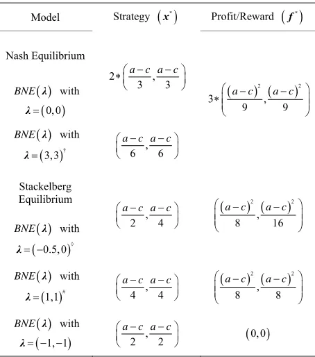
Table 1. Strategies and profits for various equilibria.
Model Strategy
x* Profit/Reward
f*Nash Equilibrium
BNE λ with
0, 0
λ
2 , 3
c
a3c a
BNE λ with
†
3,3
λ 6 , 6
ac a
c
2 2
3 , 9 9 ac ac
Stackelberg Equilibriu
m
BNE λ with 0.5
λ ,0
, 2 4
ac ac
2 2
, 8 16
a c a c
BNE λ with
1,1
λ # 4 , 4
ac ac
2 2
, 8 8
a c a c
BNE λ with 1,
λ 1 2 , 2
ac ac
0,0
†It has the same pr its as Nash equilibrium but half production. ◊It achieves
the Stackelberg equilibrium but is not Pareto-optimal. #This is the Pareto-optimal equilibrium.
of
*
a
r *
* *
d d d d
1 and 1,
d d
d d
B B
a b
a b
a b
r r r
x x
x x
b
(4 )
and the b unctions are perfect in terms of repre- senting the reality. Unfortunately, the profits r both players at the equilibrium will be , showing that if
le, we also included the case with 2
elief f
fo
0
both players are perfectly smart, the outcome could be a tragedy.
In this tab 3
w the which interestingly results in the same profits a
equilibrium but with half production. To show ho s the Nash
belief (or the interference derivative ) affects the strategy * * *
a b
x x x and the reward f* fa* fb*, we
provide the results in Figure 1 assumi g that n a c 10.
3.4. Existence
Since the birth of game theory, the quest for the existence of an equilibrium has been the focal point in this area. In [6], Nash proved the existence of the widely known Nash equilibrium we know today. Later, numer us researchers presented further theorems and proofs about xist- ence of the game-theoretic equilibria [7,8]. n
o
the e Based o the literature, we provide the sufficient existence of the general BNE game. what is known in
condition for the
Corollary 1 Consider a K-player game, with the strategy spaces k for k1, 2, , K, which are not empty, compact and convex subsets of an Euclidean space. If the predicted reward function
, B , t
k k k k k
f x r x x k is continuous and quasi-concave in Sk for any fixed
t k
[image:6.595.308.536.469.686.2]x , then there exists an equi- librium.
Figure 1. The strategy and reward at various equilibria
against the belief assuming . The solid line
refers to the resul s for the str e the dash line shows the rewards.
λ
t
Proof The BNE game (with forward-looking players) presented in Section 3.2 follows the same spirit as a typical Nash game where any player acts towards an equilibrium assuming that other players’ strategies are fixed. Their only difference lies in their understanding about the payoff functions due to different level of cog- nition to the environment. Consequently, the same result regarding existence of Nash equilibrium [7] can be di- rectly applied to BNE by simply replacing the pay off function by the predicted reward function, which com- pletes the proof.
4. Conclusion
This paper showed the importance of players’ cogn to the equilibrium of the game and presented the equilibrium of forward-looking players. Using a two-fi example, we demonstrated how a Nash game with belief (referred to as BNE) can be made to achieve the Nas
ition Nash rm
h and Stackelberg equilibria. On the other hand, this paper has also illustrated the potential of using the belief func- tion as an optimization parameter which makes possible the game converging to a Pareto-optimal equilibrium. However, this is a new regime in game theory and future work is required to better understanding of belief-di- rected games.
REFERENCES
[1] M. J. Osborne and A. Rubinstein, “A Course in Game Theory,” MIT Press, Cambridge, 1994.
[2] G. H. Von Stackelberg, “Market Structure and Equilib- rium,” Springer-verlag, Berlin, Heidelberg, 2011.
http://dx.doi.org/10.1007/978-3-642-12586-7
[3] E. Rasmusen, “Game and Information,” Basil Backwell Ltd., Oxford, 1989.
[4] J. Nash, “Non-Cooperative Games,” The Annals of Ma- thematics, Vol. 54, No. 2, 1951, pp. 286-295.
http://dx.doi.org/10.2307/1969529
[5] D. Fudenberg and J. Tirole, “Game Theory,” MIT Press, Cambridge, 1991.
[6] J. Nash, “Equilibrium Pints in n-Person Games,” Pro- ceedings of the National Academy of Science, Vol. 36, No. 1, 1950, pp. 48-49.
http://dx.doi.org/10.1073/pnas.36.1.48
[7] D. A. Debreu, “Social Equilibrium Existence,” P ings of the National Academy of Science, Vol.
roceed- 38, No. 10,
073/pnas.38.10.886
1952, pp. 886-893.
http://dx.doi.org/10.1