A Comparison between Evolutionary Metaheuristics and Mathematical Optimization to Solve the Wells Placement Problem

A Comparison between Evolutionary Metaheuristics and

Mathematical Optimization to Solve the Wells

Placement Problem

Ghazi AlQahtani, Ahmed Alzahabi, Ernee Kozyreff, Ismael R. de Farias Jr., Mohamed Soliman Texas Tech University, Lubbock, USA

Email: [email protected], [email protected], [email protected], [email protected], [email protected]

Received August 17,2013; revised September 20, 2013; accepted October 4, 2013

Copyright © 2013 Ghazi AlQahtani et al. This is an open access article distributed under the Creative Commons Attribution License,

which permits unrestricted use, distribution, and reproduction in any medium, provided the original work is properly cited.

ABSTRACT

The Wells Placement Problem (WPP) consists in choosing well locations within an oil reservoir grid to maximize the reservoir total oil production, subject to distance threshold between wells and number of wells cap constraints. A popu-lar approach to WPP is Genetic Algorithms (GA). Alternatively, WPP has been approached in the literature through Mathematical Optimization. Here, we conduct a computational study of both methods and compare their solutions and performance. Our results indicate that, while GA can provide near-optimal solutions to instances of WPP, typically Mathematical Optimization provides better solutions within less computational time.

Keywords: Wells Placement; Genetic Algorithm; Integer Programming

1. Introduction

Consider an oil reservoir for which oil production totals over the entire reservoir area are given (or estimated). We are interested in the Wells Placement Problem (WPP), i.e., the problem of maximizing the total oil pro-duction of the reservoir by selecting locations to build at most a certain number of vertical wells at a given mini-mum distance apart from one another.

WPP (and variations of it) has been the subject of a number of studies in the last decades [1-9]. The main approaches used to find solutions have been Genetic Al-gorithms (GA), which are a special type of Evolutionary Metaheuristics, and Integer Programming (IP), a subclass of Mathematical Optimization.

To the best of our knowledge, the earliest study of wells placement optimization using IP was the work conducted in 1974 by Rosenwald and Green [8], who developed a numerical optimization framework to select optimal positions of wells. Their objective was to mini-mize the difference between actual and desired flow curves by choosing optimum well locations from prede-fined location sets. In 1997, Vasantharajan and Cullick [9] introduced the term reservoir quality to represent reser-voir connectivity adjusted by tortuosity, which was the surface area surrounding the flow by the volume con- tained. The well site selection process was performed

through IP, with the goal of maximizing reservoir quality. Later, in 1999, Cullick et al. [4] improved the formula-tion of the problem by reducing its number of con-straints.

Some of the articles cited above report computational results using either GA or IP, but we are not aware of a study that compares both. In this paper, we use GA and IP to solve instances of WPP, and report the computa-tional results of those tests.

Specifically, our test reservoir sits on an m n grid, where each of the sites in the grid represents a pos-sible location for a well. For each , where

mn

 

i j,  I J



1, ,



I   m and J 



1, , n



D

, a production total  i j, is associated with the site, and each pair of sites

chosen needs to be at least grid units apart from each other. Finally, the maximum number of well loca-tions selected, , is predetermined.

p

N

2. Evolutionary Metaheuristics

Evolutionary Metaheuristics use ideas of biology and Darwin’s theory of evolution, such as reproduction, mu-tation, and “survival of the fittest”, to provide solutions to problems that arise in other fields of study. Because one of the most used types of evolutionary metaheuristics in petroleum engineering is genetic algorithms, we veloped a GA to tackle our problem of interest (for de-tails on the structure and use of GA in general, see [10]).

2.1. Definition of Terms and Variables

Our GA starts with an initial population that is improved through crossover, local search, mutation, and the addi-tion of new members to the populaaddi-tion, which we call intruders. After a generation, the best fit individuals of the population are selected, the others are discarded, and a new generation begins. The algorithm runs for a prede-termined number of generations, ng, and returns the fittest individuals of the final population. The fitness of an individual, here, is the total oil production associated with it.

An individual z

y is represented by an -array of

ordered pairs (which we call coordinates), and denoted as

N



 









1, 1 , 2, 2 , , ,



z

z z

z

N N

y  i j i j  i j

where



,



z

N N

i j , , represent the locations

on the grid of the wells defined by



1, ,

k  N



z

y . Associated with

z

y , the value pz is the total oil production that results from choosing this individual, given by Equation (1).

 

1 _, z

k k

N

z k _{i j}

p 



 p (1)

We denote the production totals matrix by , i.e., an element of row i and column of is

 i j, , and we define (0,0) We let be the sorted

vector of the elements of and its corresponding co- ordinates:

m n P

j p

p p 0

P

q



























1, ,1 1 , 2, 2, 2 , , mn, mn, mn



q q r s q r s  q r s

where

1 2 mn

q q q ,

_k,_k

k r s

q  p _, and











r s1, 1 , , rmn,smn



 I J.

2.2. The Genetic Algorithm

The high level structure of our GA is as follows:

At each generation g, np is the number of indi-viduals in the initial population, c is the number of crossover operations performed, and i is the number of intruders created. The value is used in the sub-routine LOCAL-SEARCH, and will be explained

later.

n

n

Lines 1 - 5 initialize the variables of the algorithm, which are the individuals of the population, at zero. Line 6 creates the initial population, and lines 7 - 12 perform evolutionary sub-routines for ng generations. Finally, line 13 returns the best fit individual found.

t

y

This routine takes as input an individual, , and re-turns 1 if the individual is feasible, or 0 ot ise. The procedure simply computes the Euclidea be-tween every pair of coordinates that define the individual, and checks whether the distance is at least

herw n distance

.

D

The routine INITIAL-POPULATION can be divided

into two main blocks: lines 1 - 12 and 13 - 29. The first block creates a “greedy” solution to the problem by choosing the coordinates of 1

y , the first individual of the population, based on th of sorted values of . The second block creates the rest of the initial po lation by selecting ran on the grid (usi the function

e vector

dom q

locations P

pu

ng rand( )A , which returns a random ele ent of a finite set m A), with the condition that each individual created is feasible.

We note that, for large values of , it may be hard, and perhaps even impossible, to locations on the grid such that the minimum ween each pair of locations is Our algorit kes

at-mpts to find such locations, and, in t o

N find distance bet

hm h

N

ma e

D. 10N

case that it is te

n t successful, some of the coordinates of the individual being created remain as

 

0,0 .

The sub-routine CROSSOVER performs the

repro-duction of individuals. In this routine, two individuals of the population 1_{, ,} np

y  y are selected at random (lines 2 - 3), and the crossover point, represented by d, is also selected at random (line 4). In lines 5 - 12, the crossover occurs, and two new individuals are created. These new

individuals are then c for feasibility, and, in the case that they are not feasible, they are “erased” from the population by setting all of th

hecked

eir coordinates to

 

0,0 (lines 13 - 21). The procedure is repeated nc times, and the routine creates 2nc new individuals.

n the dual of Our GA then s a local search in the grid, i geographical sense, to try to improve ever indivi the population.

perform

y

at random, and, in case it is not , a local search in the reservoir grid, within a s

 

area

0, 0

quare of



2Δ1



2 centered at



,



z

i j

search ar

, is perform to fin tion in the ea such

ed to try that, if substituted in

d a loca- place of



,



z

i j

increase

, will maintai sociated

n feasib its as

ility of the individual and

z

p ch fo

value the m

1_{, ,} ost. The

th r

routine performs is local sear np2nc

m wh

vid th

y  y

utation, ual of

, a

xt p is ic

d f ery di e p

nd returns

h, again, is opulation their updated

The ne performe

1_{, ,}

values. genetic o or ev

2

erator in

p c

n n

. y  y 

This routine picks a coordinate  from individual z

y at random and replaces it with another co

picked at random the entire grid. If the replacement keeps

ordinate in

z

y feasible and improves the value of pz, then

z

y is updated; otherwise, z

y remains unchanged. Our last genetic operator, INTRUDERS, creates ni individuals that enter the population “ utside”. The intention of this proc

fr is to add

om o

edure variability to the population thus far created.

This routine is similar to INITIAL-POPULATION.

choice o the coordinates of the new individuals more ective: they are chosen a ng the top 10N value

The main differences are in 6,

f is

sel mo s of

th a

and preserves the

lines 2 and where the

e P matrix. Thus, this routine brings to the popul

-tion not only variability, but also members with high fitness.

Our final sub-routine selects np

2

best t individuals from the entire population

fi 1_{, ,} np nc ni

y  y   , which will become the initial population of

eration.

the next

gen-The sorting procedure in line 1 is, in fact, a renumber-ing of the individuals 1_{, ,} np 2nc ni

y  y   based on the values pz, 



1, , p2ncni



give as input z  n

e we

. As a clarifying

example, suppos to this line

   



3, 4 ,



1_{ 1, 2 ,}

y y2



   

5,6 , 7,8



, and



 







3_{ 9,10 , 11,12 , with}

1 10

p  , p2 30

y  , and

3 20

p  . Then the output will be y1



   

5,6 , 7,8



,



 







2 _{9,10 , 11,12}

y  , and y3



   

1, 2 , 3, 4



. Lines 2 - 7 simply erase variables np 1, , np 2

y   y  and keep

1_{, ,}

c i

nn

p

n

y  y which are the surviving individuals that will start a new generation. (In case gn_g, then there will not be another generation, and WPP-GA will return 1

individual with the best fitness found after

y,

the ng

gen-erations.)

A careful analysis of WPP-GA and its sub-routines

shows that the algorithm terminates, but not necessarily ith an optimal solution to the problem, i.e., an individ-ual whose fitness is the highest possible.

3. Mathematical Optimization

Mathematical Optimization approaches quantitative problems using tools such as linear algebra, calculus, and graph theory. In a sense, it is a more sophisticated me-thod than Evolutionary Metaheuristics, and, in practice,

sually requires bigger and more structured algorithms to

case, IP, is tha

i

It is common practice, in IP

defining an objective to be m ized (

nimized fine the problem i

question. Here, the for n of WPP is as fo w

u

solve a given problem.

The main advantage of using mathematical optimiza-tion, and, in our particular t a solution may be proven to be optimal, as opposed to GA, which does not guarantee opt mality of the best solution found.

, to formulate problems by

function axim or

mi-), subject to constraints that de n

         







 

 



 i j, 0,1

 

, ,

x  i j  I J

where a variable _{ }i j,

 

, ,

i j

1 1 1 2

, ,

1 1 2 2

, , 2 2

1 2

,

1 2

maximize , ,

subject to 1,

i j i j I J

i j i i j

j

p x

i j I J

x x

i i j j D

        _     



x represents the location

 

i j, in

the oil reservoir grid, and is equal to 1 if the location is chosen, or 0 otherwise. Hence, a feasible soluti this

h

shown. Note that

EX 12 with default settings, except for the search strategy, which was set to Traditional Branch-and-Cut, and the relative and absolute gap tolerances, which were set to zero. Every test had a time limit of 3600 seconds.

Our test grid has , and we set the values

of to h of these values,

we tried to solve set to , up to

the nt at limi

et on to at satisfies all problem is a mn-vector of 0’s and 1’s t

constraints defined in the formulation

this is a completely different way of representing a solu-tion, in comparison with our GA. Nonetheless, the values of the objective function, here, and the fitness of the in-dividuals, in the GA, are comparable, since they have the same meaning.

To solve our instances with the IP approach, we use a commercial solver based on branch-and-cut that can handle large-scale optimization problems. For details on branch-and-cut, the reader is referred to [11].

4. Computational Tests

We ran our computational tests in the Texas Tech High Performance Computing Center’s 3.0 GHz CPUs with 16 GB RAM nodes. For the tests using IP, we used CPL

100

m n

, and 20. For eac WPP with N

which either the time as

D

poi

8, 12, 16

w

10, 20, t was reached, or

m the value of N not reached, i.e., neither hod was able to find a solution that represented N well

lo-cations. For the GA, we set ng 10000, np1000, 100

c

n  , n_i , and  10 for all tests.

The values of the P matrix were obtained with the

commercial reservoir simulator Eclipse, using the Qual-ity Maps approach (see [12] for details). Some main cha-racteristics of our heterogeneous and anisotropic reser-voir are: initial pressure of 4000 psi, porosity of 22%,

and horizontal 10 

perm of with

st

eability average 175mD

andard deviation of 91.1mD. The distance between

two closest grid points is 300 ft, and the thickness of

the reservoir is 75 ft.

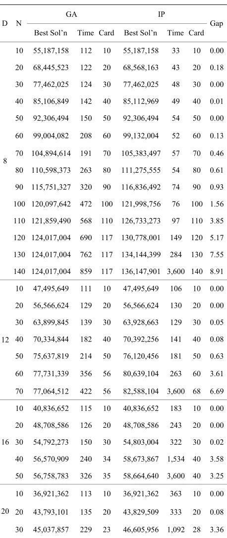
Table1 shows the results obtained using both GA and

displays the value of the ethods. (Note: in GA, this

nality of the solution found, i.e., t

ated wi so

een the G

IP. The columns “Best Sol’ n” best solutions found by both m

value is called the fitness of the best individual, whereas in IP it is called the objective function value of the best solution. We will use the latter expression in our analy-sis.) “Time” shows the computational time, in seconds,

required for the test to finish. We note that, because of the settings used in CPLEX, all solutions obtained using IP are provably optimal precisely when the time is less than 3600 seconds. The column “Card” shows the

cardi-he number of well loca-tions associ th that lution. Finally, “Gap” refers to the relative percentage difference betw A and IP best solutions, and is computed using Equation (2).

’ ’

Best Sol n with IP Best Sol n with GA

Gap 100

Best Sol n with IP’ 

 

) (2

he best

From Table1, it is clear that the problem gets harder

as the values of D and N increase. On the IP section

of the table, this is reflected in the time required to solve the instances. On the GA side, both the computational time and the cardinality of solution show the increase in the difficulty of the problem. For instance, for

8

D

t

 and N120, the best solution that GA can find has cardinality 117, althoug tions with greater car-dinality (and better objective

h solu

function value) do exist, as th

al software developers who worked on it for decades. The seemingly small values in the last columns reflect this contrast of algorithms: a gap as small as 0.1% can very

5.

wells in an e IP results show.

Overall, IP was capable of finding better solutions than GA, and, most of the time, was faster. In every test, the best solution found by IP had an objective function value at least as good as the one found by the GA. In 8 cases, both methods found an optimal solution to the problem, and in 11 other cases, the gap between the two methods was less than 1%. This shows that GA can be effective for instances that are less challenging, but, for the harder instances, IP was notably more successful than GA.

The merit of being faster and finding better solutions is due not only to the differences in approaching the prob-lem (IP vs. GA), but also a result of the algorithms used to solve the instances. While our GA has less than 500 lines of code, CPLEX is the product of profession

be mal difficult to close, and thus finding a sub-opti solution can be a much easier task than finding an opti-mal one. Moreover, the fact that CPLEX can guarantee the optimality of a solution is a feature that a GA does not have. It is only in comparison studies such as the present study, that one can visualize the effectiveness of a GA, in finding optimal solutions. Finally, we note that CPLEX is a multi-purpose solver that can handle a vast number of different problems, while our GA was devel-oped specifically to tackle WPP.

Conclusions and Further Research

[image:6.595.58.287.97.639.2]

Table 1. Summary of results using GA and IP.

GA IP D N

Best Sol’n Time Card Best Sol’n Time Card Gap

10 55,187,158 112 10 55,187,158 33 10 0.00

20 68,445,523 122 20 68,568,163 43 20 0.18

30 77,462,025 124 30 77,462,025 48 30 0.00

40 85,106,849 142 40 85,112,969 49 40 0.01

50 92,306,494 150 50 92,306,494 54 50 0.00

60 99,004,082 208 60 99,132,004 52 60 0.13

70 104,894,614 191 70 105,383,497 57 70 0.46

80 110,598,373 263 80 111,275,555 54 80 0.61

90 115,751,327 320 90 116,836,492 74 90 0.93

100 120,097,642 472 100 121,998,756 76 100 1.56

110 121,859,490 568 110 126,733,273 97 110 3.85

120 124,017,004 690 117 130,778,001 149 120 5.17

130 124,017,004 762 117 134,14 8

4,399 284 130 7.55

40 8.91 140 124,017,004 859 117 136,147,901 3,600 1

10 47,495,649 111 10 47,495,649 106 10 0.00

20 56,566,624 129 20 56,566,624 130 20 0.00

30 63,899,845 139 30 63,928,663 129 30 0.05

40 0.08

75,637,819 214 50 76,120,456 181 50

60 3.61

12

3, 70,334,844 182 40 70,392,256 141 40

50 0.63

77,731,339 356 56 80,639,104 263 60

70 77,064,512 422 56 82,588,104 600 68 6.69

10 40,836,652 115 10 40,836,652 183 10 0.00

20 48,708,586 126 20 48,708,586 243 20 0.00

30 54,792,273 150 30 54,803,004 322 30 0.02

40 56,570,909 240 34 58,673,867 1, 16

3,

534 40 3.58

50 56,758,783 326 35 58,664,640 600 40 3.25

10 36,921,362 113 10 36,921,362 363 10 0.00

20 43,793,101 135 20 43,829,509 333 20 0.08 20

1,

30 45,037,857 229 23 46,605,956 092 28 3.36

obj u o

the rese icate that GA

-tive for easier instances t e

har i k

app o

GA, and m h aster. More

advantage of finding provably optimal solutions, while

GA o u te a t l

The G ted re can, m

and v or c nh h t

cha n r , by d in t

ram rs y e t

faster by ng f nt form

-lem d ra o intain

both p i l e t v

parameters, to provide a basic GA, and to use a

straight-forw d n o P

As fu r g f

ventional wells placement, a more challenging problem,

sinc t th ar s ly r ,

s ire a 3 ri t o

cations for

6. A

e

n

The aut ow g e o n C

Tech U at Lubb k f r

pr v n s h e s

resu r th i p

RL: http://www.hpcc.ttu.edu

ective of extracting the maximum amo nt f oil from rvoir. Our results ind

, bu

can be e rform

ffec e for it lacks p anc der ones. In comparison, CPLEX (wh ch ta es the IP

roach) always f ost of t

und e tim

a solu e f

tion at least over, IP

as good a has the

s our

is n t able to g aran e th t a solution is op ima . A presen

e its perf he man of course anced, eit , be er by odified ac

ha e e ually

ngi g the algo ithm or simply a just g i s pa-ete . Similarl

consideri , th

dif solu ere

ion via IP ulations can of t be he p made rob an tuning some pa meters on CPLEX. T ma

a proaches s mple y, w chose no to ary those

ar formulatio for ur I approach.

rther resea ch, we su gest the study o

non-con-e i involvnon-con-es wnon-con-ells at non-con-e not nnon-con-ecnon-con-e sari vnon-con-e tical and thu may requ D-g d as the se of p ssible

lo-the wells.

cknowledg me ts

hors ackn led e th High Perf rma ce om-putin

o g C idi

enter at Texas g resource niversity contributed oc re o earch

that ave to th

lts eported wi in th s pa er. U

We thank Dr. Jerome Onwunalu’s for guidance and support, and for providing a GA code used in preliminary tests.

This research was partially supported by the Office of Naval Research (ONR) through grant N000141310041 to de Farias.

REFERENCES

[1] G. AlQahtani, R. Vadapalli, S. Siddiqui and S. Bhatta- charya, “Well Optimization Strategies in Conventional Reservoirs,” Proceedings of SPE Saudi Arabia Section Technical Symposium and Exhibition, Al-Khobar, 8-11

April 2012, 13 Pages.

http://dx.doi.org/10.2118/160861-MS

[2] O. Badru and C. S. Kabir, “Well Placement Optimization in Field Development,” SPE Annual Technical Confer- ence and Exhibition, Denver, 5-8 October 2003, 9 Pages.

[3] W. Bangerth, H. Klie, M. F. Wheeler, P. L. Stoffa and M. K. Sen, “On Optimization Algorithms for the Reservoir Oil Well Placement Problem,” Computational Geosci- ences, Vol. 10, No. 3, 2006, pp. 303-319.

http://dx.doi.org/10.1007/s10596-006-9025-7

[4] A. S. Cullick, S. Vasantharajan and M. W. Dobin, “De- ocations from a 3D Reservoir 6549879 B1, 2003.

. L. Rogers and J. J. termining Optimal Well L

Model,” US Patent No. US

[5] D. Y. Ding, “Optimization of Well Placement Using Evo- lutionary Algorithms,” SPE EAGE Annual Technical Conference and Exhibition, Rome, 9-12 June 2008, p. 912.

[6] B. Guyaguler, R. N. Horne, L

18. [7]

ent Optimization Procedures,” International Con-e and Exhibition, Abu Dhabi, 3-6 November 2008

14 Pages.

[8] G. W. Rosenw A Method for

De-ing Optimization,” Proceedings

. 421-426. 1

J. Onwunalu, M. Litvak, L. J. Durlofsky and K. Aziz, “Application of Statistical Proxies to Speed up Field De- velopm

ferenc ,

[

ald and D. W. Green, “

[12

termining the Optimum Location of Wells in a Reservoir Using Mixed-Integer Programming,” SPE Journal, Vol.

14, No. 1, 1974, 12 Pages.

[9] S. Vasantharajan and A. S. Cullick, “Well Site Selection Using Integer Programm

of IAMG’97, 22-26 September 1997, pp

10] R. Haupt and S. Haupt, “Practical Genetic Algorithms,” John Wiley and Sons, Hoboken, 2004.

[11] G. L. Nemhauser and L. A. Wolsey, “Integer and Com- binatorial Optimization,” John Wiley and Sons, Hoboken, 1988.