Using the urban landscape mosaic to develop and validate methods for assessing the spatial distribution of urban ecosystem service potential

(1)

USING THE URBAN LANDSCAPE MOSAIC TO

DEVELOP AND VALIDATE METHODS FOR

ASSESSING THE SPATIAL DISTRIBUTION OF

URBAN ECOSYSTEM SERVICE POTENTIAL

Oliver Twanhaw GUNAWAN

School of Environment and Life Sciences

College of Science and Technology

University of Salford, Salford, UK

(2)

i

List of Figures

Chapter 2

Figue 2.1. The twelve principles of the Ecosystem Approach grouped into four

themes (adapted from UKNEAFO, 2014) ... 5 Figure 2.2. Ecosystem service cascade model (CICES, 2013). ... 8 Figure 2.3. Evolution of ecosystem service classifications. The colours represent the

evolutionary path of the supporting (purple), provisional (orange), regulation and maintenance (green) and cultural services (blue) and are taken from the CICES classification (Haines-Young and Potschin, 2010). ... 11 Figure 2.4. Revised ecosystem service framework (Author’s own - amended from

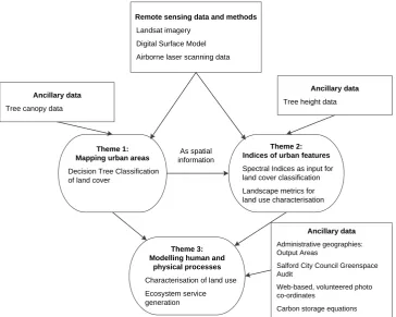
Bastian et al., 2012). ... 12 Figure 2.5. Three interrelated themes describing how remote sensing data and

methods support research in global environmental change

(from Wentz et al., 2014). ... 27 Figure 2.6. Flow diagram of overall thesis structure ... 35

Chapter 3

Figure 3.1. Overall thesis structure. ... 39 Figure 3.2: Map of Salford. This work is based on data provided through EDINA

UKBORDERS with the support of the ESRC and JISC and uses boundary material which is copyright of the Crown (2015). ... 41 Figure 3.3. Salford (shaded in grey) as part of Greater Manchester (white). Black

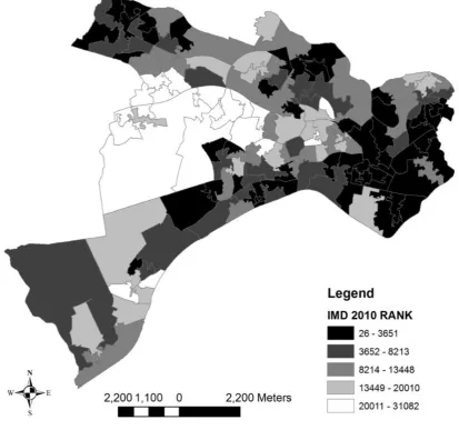
outlines represent Administrative Lower Super Output Areas. This work is based on data provided through EDINA UKBORDERS with the support of the ESRC and JISC and uses boundary material which is copyright of the Crown (2015). ... 42 Figure 3.4. The ranked index of Multiple Deprivations (IMD) 2010. Black outlines

represent Administrative Lower Super Output Areas. Low values indicated by darker shading represent the most deprived areas, while higher values

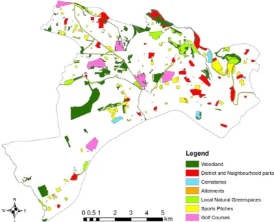
shaded in lighter greys represent the least deprived nationally. Values are ranked such that 1 is the most deprived. This work is based on data provided through EDINA UKBORDERS with the support of the ESRC and JISC and uses boundary material which is copyright of the Crown. ... 43 Figure 3.5. Greenspaces audited by Salford City Council. (SCC, 2006) ... 44 Figure 3.6. Remote sensing structure adapted from Wentz et al., (2014) to include

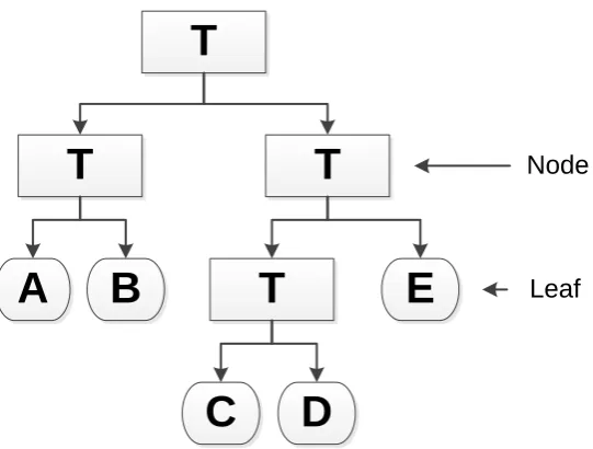
features specific to this research. ... 50 Figure 3.7. Representation of a Decision Tree Classification system. T represents the

(9)

viii Chapter 4

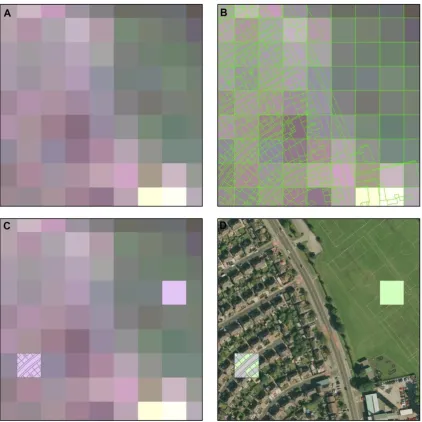
Figure 4.1: Datasets used within each component of the thesis. ... 72 Figure 4.2. Comparison of sample pixels and aerial photography (A) Landsat

imagery, (B) Overlaid, gridded OSMM data, (C) Selection of sample pixels, (D) Overlaid aerial photography (Landmap; The GeoInformation Group 2007). ... 78 Figure 4.3. Example of building height data extracted from LiDAR (A), LiDAR height

information (light pixels indicate higher features), (B) LiDAR data with derived building footprints, (C) footprints overlaid onto aerial photography. (Landmap; The GeoInformation Group (2014), Landmap; The GeoInformation Group, 2007) ... 80 Figure 4.4. Example of tree height data. LiDAR height information (light pixels

indicate higher features), (B) LiDAR data with tree canopy footprints, (C) Building footprints overlaid onto aerial photography. (Landmap; The

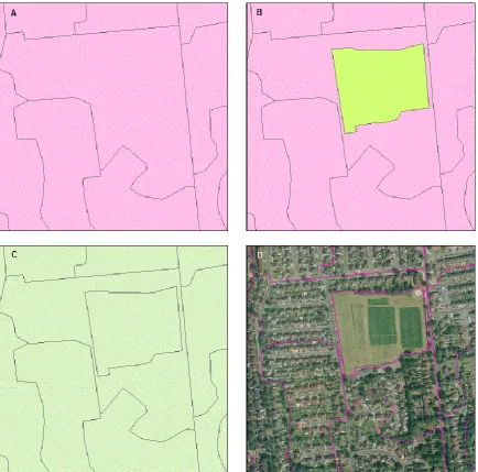
GeoInformation Group 2007) ... 81 Figure 4.5. Integration of 2 ha green spaces into OA layer. (A), OA layer, (B) overlaid

green spaces, (C) union function, (D) final product overlaid onto aerial

photography (Landmap; The GeoInformation Group 2007). ... 83 Figure 4.6. Screen grab from geograph.org showing the number of photos captures

in 100 m grid centisquares across a section of Salford (Geograph Project Ltd, 2012). ... 85 Figure 4.7. Field survey sample sites for cultural and carbon storage service

validation (Author’s own) ... 89

Chapter 5

Figure 5.1. Flow diagram of land cover mapping methodology. ... 94 Figure 5.2. Spectral index value ranges by land cover type as identified by sample

points taken from OS MasterMap and 2006 aerial photography. Column headings refer to the spectral indices used. These are listed in Table 3.5 (Author’s own). ... 96 Figure 5.3. Polygons representing the frequencies of pixel values by land cover type. (A) NDVI, (B) MSAVI, (C) NDWI, (D) MNDWI, (E) NDBaI, (F) NDBI, (G) UI, and (H) IBI (Author’s own). ... 97 Figure 5.4. Reclassified water images from (A) NDWI, (B) MNDWI, (C) NDBaI

and, (D) OS MasterMap reference data (Author’s own). ... 98 Figure 5.5. Reclassified peat images from (A) NDBI, (B) MNDWI, and (C) UI

(Author’s own). ... 100 Figure 5.6. Decision tree classification rules for broad land cover classification. White

boxes contain the rules applied at each stage of the decision tree

classification. Grey boxes contain the name of the final land cover classes. ... 103 Figure 5.7: The final decision tree classification. White boxes contain the rules

(10)

ix Figure 5.8. Decision tree classified map using index-based bands (Author’s own). 107 Figure 5.9. Maximum likelihood classified map using raw Landsat bands

(Author’s own). ... 108 Figure 5.10. Final classified image (Author’s own). ... 110 Figure 5.11. Comparison of differing green space estimates. Positive percentage

change shows that remote sensing classification identified more green space than that presented by the audit (Author’s own). ... 113 Figure 5.12. Flow diagram of land use characterisation methodology ... 115 Figure 5.13. Moving window diameter against maximum landscape metric scores (A)

SIDI, (B) Mean Euclidean nearest neighbour, (C) Mean patch size of

buildings and, (D) Patch size standard deviation of buildings. ... 117 Figure 5.14. Characterisation of urban land use (Author’s own)... 121 Figure 5.15. Landscape scores for the representative central point of each cluster 122 Figure 5.16. Histogram of ‘detached’ cluster distances from the central point of the

cluster ... 123 Figure 5.17. Histogram of ‘semi-detached’ cluster distances from the central point of

the cluster ... 124 Figure 5.18. Histogram of ‘terraced’ cluster distances from the central point of the

cluster ... 124 Figure 5.19 Histogram of ‘non-domestic’ cluster distances from the central point of

the cluster ... 125 Figure 5.20. Histogram of ‘agricultural’ cluster distances from the central point of the

cluster ... 125

Chapter 6

Figure 6.1. Methodology for Chapter 6. ... 130 Figure 6.2. Water mitigation surface based on Chapter 5 land cover map

(Author’s own). ... 133 Figure 6.3. Path-distance analysis ignoring potential mitigating properties of

Chapter 5 land cover map (Author’s own). ... 134 Figure 6.4. Path-distance analysis including land cover-based water flow mitigation

properties (Author’s own). ... 135 Figure 6.5. Carbon storage ecosystem service generation layer (Author’s own)... 141 Figure 6.6. Water flow mitigation ecosystem service generation layer (Author’s own).

... 141 Figure 6.7. Climate stress mitigation ecosystem service generation layer

(Author’s own). ... 142 Figure 6.8. Recreation ecosystem service generation layer (Author’s own). ... 142 Figure 6.9. Aesthetics ecosystem service generation layer (Author’s own). ... 143 Figure 6.10. Correlation between tree heights from ecosystem service layer and field

survey. ... 144 Figure 6.11. Correlation between derived carbon stored from ecosystem service layer

(11)

x Figure 6.12. Correlation between water flow mitigation derived through the

ecosystem service layer and STAR tools. ... 146 Figure 6.13. Correlation between water flow mitigation derived through the

ecosystem service layer and STAR tools, considering total LSOA volumes of surface water runoff. ... 147 Figure 6.14. Correlation between climate stress mitigation derived through the

ecosystem service layer and STAR tools. ... 148 Figure 6.15. Carbon storage hotspots. Aspatial hotspots are outlined in red.

Spatial hotspots are shaded in greyscale (Author’s own). ... 151 Figure 6.16. Water flow mitigation hotspots. Aspatial hotspots are shaded in black

(Author’s own). ... 152 Figure 6.17. Climate stress mitigation hotspots. Aspatial hotspots are outlined in red.

Spatial hotspots are shaded in greyscale (Author’s own). ... 153 Figure 6.18. Recreation hotspots. Aspatial hotspots are outlined in red. Spatial

hotspots are shaded in greyscale (Author’s own). ... 153 Figure 6.19. Aesthetics hotspots. Aspatial hotspots are outlined in red. Spatial

hotspots are shaded in greyscale (Author’s own). ... 154

Chapter 7

Figure 7.1. Methodology for Chapter 7.The grey boxes indicate themes of analysis. The top grey box encapsulates the ecosystem service generation layers created in Chapter 6. The bottom two grey boxes encapsulate the Aspatial and Spatial methodologies. ... 162 Figure 7.2. An example of silhouettes for 2 – 4 cluster solutions. Rows of dots

represent the ‘silhouettes’ of individual members of a cluster compared to the centre of the cluster (from Rousseeuw, 1987). ... 164 Figure 7.3. Boxplots displaying normalised ecosystem service generation values by

landscape character (A) Terraced, (B) Semi-detached, (C) Detached,

(D) Non-domestic, (E) Agriculture, (F) Woodland, and (G) Green or blue. . 169 Figure 7.4. Significant differences in ecosystem service generation between

landscape character pairs. Shaded rectangles indicate paired character types that displayed significantly different patterns (p < 0.01) for: orange =

Aesthetics, red = Climate stress mitigation, green = Carbon storage, blue = water flow mitigation, and purple = recreation. White rectangles represent no correlate between ecosystem service pairs. ... 170 Figure 7.5. Hotspot congruence for (A) aspatial and (B) spatial hotspots (p < 0.1)

(Author’s own). ... 174 Figure 7.6. The deviation in cluster size from the mean. (A) Aspatial clustering, (B)

Spatial clustering. ... 175 Figure 7.7. Average distances from cluster centres for spatial and aspatial cluster

(12)

xi Figure 7.10. Geographical distribution of ecosystem service generation clusters -

Aspatial approach (Author’s own). ... 182 Figure 7.11. Geographical distribution of ecosystem service generation clusters -

Spatial approach (Author’s own). ... 183 Figure 7.12. Box plots of the ecosystem service values in each cluster for aspatial

bundling ... 184 Figure 7.13. Box plots of the ecosystem service values in each cluster for spatial

bundling ... 185 Figure 7.14. Greenspaces as identified using three approaches; from the SCC

greenspace audit and from aspatial and spatial hotspots created in chapter 6 (shaded grey). Areas shaded green are highlighted in all three approaches (Author’s own). ... 189

Chapter 8

Figure 8.1. Cartographic model of methodology for Chapter 8. ... 195 Figure 8.2. Greenspace entrance points (yellow) around the perimeter of Buile Hill

Park, Salford (green). The park centroid is shaded in red. (Landmap;

The GeoInformation Group 2007) ... 196 Figure 8.3. SCC Service Areas (Light grey) and ANGSt Service areas (Dark grey)

(Author’s own). ... 201 Figure 8.4. Percent of addresses inside (A) SCC service areas and (B) ANGSt

service areas by ward (Author’s own). ... 202 Figure 8.5. ANGSt greenspace physical accessibility based on the ANGSt service

areas. Values are hectares per 1000 population. Population is based on an estimation of 2.3 people per address (ONS, 2014) (Figure is Author’s own). ... 204 Figure 8.6. SCC greenspace physical accessibility based on SCC service areas.

Values are hectares per 1000 population. Population is based on an

estimation of 2.3 people per address (ONS, 2014) (Figure is Author’s own). ... 205 Figure 8.7. 2 ha greenspace visibility. Values represent the average number of

observers that can see the greenspace based on 100 m2 cell-level

observation counts (Author’s own)... 205 Figure 8.8. Accessible landscape: red only visually accessible, yellow only physically

accessible, green accessible both visually and physically (Author’s own). . 206 Figure 8.9. Building heights across Salford (Author’s own). This work is based on

data provided through EDINA UKBORDERS with the support of the ESRC and JISC and uses boundary material which is copyright of the Crown

(2015). ... 209 Figure 8.10. Visibility of Salford City Council audited 2 ha greenspaces at (A) ground

floor level, (B) 2nd floor, (C) 6th floor, and (D) 15th floor. Values are the average number of observers that can see the greenspace based on

(13)

xii Figure 8.11. Percentage of addresses falling within accessibility service areas at

walking speeds of 1 mps and 1.34 mps using the SCC-audited greenspaces and applying ANGSt and SCC service areas. ... 216 Figure 8.12. Increase in accessible population when walking speed is increased from 1 mps to 1.34 mps using SCC audited greenspaces (Author’s own). ... 216

Chapter 9

(14)

xiii

List of Tables

Chapter 2

Table 2.1. Open space accessibility standards for households to their closest

neighbourhood/district park (2 ha +) for each of the ten local authorities that make up Greater Manchester and Natural England’s ANGSt guidelines for

2 ha + greenspaces. ... 24

Chapter 3 Table 3.1. Methods used in the thesis. Numbers within the table refer to thesis chapters and sections. ... 40

Table 3.2. Area of greenspace by type over Salford (data from SCC Greenspace Audit, 2006) ... 44

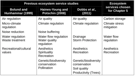
Table 3.3. Important ecosystem services in urban areas. ... 46

Table 3.4. General Land Use Database (GLUD), National Land Use Database (NLUD) land use classifications and Land use types selected for this research. ... 52

Table 3.5. Spectral indices commonly used or created for use in urban areas. Data based on articles found through a Web Of ScienceTM searchof five leading remote sensing journals from 2003 to 2013 that include the terms “urban”, “built” or “impervious” and the index abbreviation in the article title. ... 59

Table 3.6. Landscape metrics used in the landscape characterisation. From McGarigal and Marks, (1994). ... 61

Table 3.7. Contingency table for equation 3.1 ... 64

Table 3.8. Land cover, land use and ecosystem service typologies used in this research. ... 70

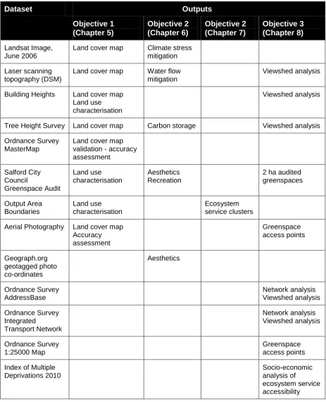
Chapter 4 Table 4.1. Raw datasets used in this thesis and the research outputs they were used to develop. ... 73

Table 4.2. Landsat TM spectral information ... 75

Table 4.3. Field Survey for aesthetics services ... 90

Table 4.4. Field Survey for recreation services ... 90

Chapter 5 Table 5.1. Accuracy assessment for water classification using NDWI, MNDWI and NDBaI. ... 99

Table 5.2. Accuracy assessment for peat using NDBI, MNDWI and UI ... 100

Table 5.3. Accuracy assessment for vegetation using NDVI and MSAVI ... 101

Table 5.4. Accuracy assessment for impervious surfaces using NDBI, UI and IBI .. 101

Table 5.5. Decision tree Index-based accuracy matrix ... 109

(15)

xiv Table 5.7. Kappa scores for the maximum likelihood and decision tree classification

... 109 Table 5.8. Final land cover map accuracy assessment ... 111 Table 5.9. Kappa values for 8 class land cover map ... 111 Table 5.10. Cluster area information. From left to right, the columns present the land

use type, the number of OAs, the average OA Area, and the total area

expressed in square metres and as a percentage of Salford. ... 120 Table 5.11. Descriptive statistics for landscape metrics in each cluster. The paired

columns for each land use type present information on the mean and

standard deviation of landscape metric values. ... 122

Chapter 6

Table 6.1. Average temperatures (K) across land cover types in Salford ... 136 Table 6.2. Weighting table for Aesthetic and Recreation Ecosystem Service

Generation (scale of 1-5) ... 137 Table 6.3. Kolmogorov-Smirnov test for normality ... 140 Table 6.4. Moran’s I statistic for spatial autocorrelation applied to each of the

ecosystem service generation layers ... 143 Table 6.5. Correlations for percentage water flow by land use type. Rows in bold are

significant at p < 0.01. ... 146 Table 6.6. Correlations for volume of water flow per LSOA by land use type.

Rows in bold are significant at p < 0.01. ... 147 Table 6.7. Correlations for average temperature per LSOA by land use type.

Rows in bold are significant at p < 0.01. ... 148 Table 6.8. Correlation between recreation measurements derived through the

ecosystem service layer and from the field survey by land character type . 149 Table 6.9. Correlation between aesthetics measurements derived through the

ecosystem service layer and from the field survey by land character type . 149 Table 6.10. Hotspot areas across Salford (m2) ... 150 Table 6.11. Overlap of spatial and aspatial hotspots for each ecosystem service.

Cell values are the hotspot areas shared expressed as a percentage of the total hotspot area. ... 151 Table 6.12. Percentage of hotspot area by landscape character - aspatial ... 155 Table 6.13. Percentage of hotspot area by landscape character - spatial ... 155

Chapter 7

Table 7.1. Ecosystem service hotspot cell recode values ... 163 Table 7.2. The effects of changing the edge detection threshold on the number of

segments produced (other variables set to default). ... 167 Table 7.3. Interquartile range values for ecosystem services (columns) by

landscape character types (rows). ... 168 Table 7.4. Pearson’s correlation of ecosystem services. No correlations were

(16)

xv Table 7.6. Shared area as a percentage of the smallest service coverage. ... 173 Table 7.7. Hotspot congruence expressed as a percentage of the total study area.

... 173 Table 7.8. Aspatial clustering solution – cells present ecosystem service values at

cluster mean centres. High values represent high ecosystem service levels (0 – 1). ... 178 Table 7.9. Aspatial clustering solution – cells present ecosystem service values at

cluster mean centres. High values represent high ecosystem service levels (0 – 1). ... 178 Table 7.10. Composition of land character types by service cluster (percent land

cover).Rows represent cluster numbers. Columns represent landscape character types. Each landscape character type has values for A = Aspatial clustering, S = Spatial clustering. Bold figure highlight dominant landscape character types (over 50%) ... 179 Table 7.11. Aspatial cluster similarities against landscape character types.

Bold figures indicate distinguishing features. ... 180 Table 7.12. Spatial cluster similarities against landscape character types.

Bold figures indicate distinguishing features. ... 180

Chapter 8

Table 8.1. Descriptive statistics for greenspace access points... 197 Table 8.2. Observer heights used in viewshed analysis ... 199 Table 8.3. Percentage of addresses within accessibility guidelines based on SCC

service areas and ANGSt service areas for The Accessible Natural Greenspace Standard (ANGSt) and the Salford City Council (SCC)

guidelines. ... 203 Table 8.4. Percentage of addresses with physical access to an ecosystem service

by land use. Values in the table represent the mean average of percentages by OA. ... 204 Table 8.5 Accessibility statistics by area of Salford across the top row (km2),

and percent of Salford’s area across the bottom row ... 207 Table 8.6. Area (km2) of physically accessible and visible greenspace across Salford.

The columns represent the area of land classified as Green and Not Green using the land cover map created in Chapter 5 ... 207 Table 8.7. Mean percentage of greenspace physically accessible or visible for

buildings outside and inside different accessibility service areas. ... 207 Table 8.8. Mann-Whitney statistics and accompanying effect sizes (p < 0.01) ... 208 Table 8.9. Number of buildings of different height located inside and outside of SCC

and ANGSt service areas. Percentages are calculated by building height. 209 Table 8.10. Spearman’s rank correlation for different view heights. All correlations

significant at p <0.01. ... 211 Table 8.11. Area (km2) of total greenspace visible at different observation heights.211 Table 8.12. Percentage land cover accessible within residential service areas and

(17)

xvi percentage of a given land cover type (column) that is physically accessible and visible from a given observer height (row). ... 212 Table 8.13. Median values for IMD and Mann-Whitney statistics with effect sizes.

For the IMD columns, lower values are more deprived. Areas shaded grey are significant at p < 0.05... 213

Chapter 9

Table 9.1. Average ecosystem service scores for populations inside and outside physical accessibility thresholds form individual residences. ... 232 Table 9.2. Overlap analysis of physically accessible spaces (5 minutes’ walk from

(18)

xvii

Acknowledgements

Firstly, I would like to thank my supervisors, Doctor Richard Armitage and Professor Philip James for their tireless support, encouragement and occasional threats throughout the last four years. I would like to thank the School of Environment and Life Sciences at the University of Salford and UNIGIS for joint funding of my

Graduate Teaching Assistantship. I would also like to thank the School for funding my attendance and participation in a number of national and international conferences through their Post Graduate Research Fund.

Secondly, I would like to thank the people and organisations who have assisted my research: Mike Savage from Red Rose Forest for supplying the Bluesky tree survey data, Steve Davey from Salford City Council for supplying the council’s greenspace audit data and the Ordnance Survey for supplying AddressBase data for Salford.

Thirdly, I would like to offer thanks to my fellow PhD candidates, past and present, in the Ecosystems and Environment research group and my fellow Graduate Teaching Assistants. I have learned so much from you and am blessed to have shared my experiences with you all. In particular, I am thinking of Alberto, Vishal, Turkia, Oliver, Chunglim, Damien, Carly, Louise, Lucy, Barbara, Calum, Ewa and Stephen.

Finally and perhaps most importantly, I would like to offer heartfelt thanks to my family who have provided much needed support of a more personal and emotional nature over the last four years. In particular I want to thank my wife Kirstine, who has had to manage the rest of our lives, and her own teaching career throughout the course of my studies. She has done so without complaint and without her belief in me, I would not have even started this research. She deserves half of this PhD, but she already has one of her own.

(19)

xviii

Abbreviations

ANGSt - Accessible Natural Greenspace Standards ANN - Artificial Neural Networks

ARIES - Artificial Intelligence for Ecosystem Services

CICES - Common International Classification of Ecosystem Services DBH - Diameter at Breast Height

DEFRA - Department of Environment, Food and Rural Affairs

DN - Digital Number

DSM - Digital Surface Model DTM - Digital Terrain Model

ED - Edge Density

ENN - Euclidean Nearest Neighbour

ETM+ - Enhanced Thematic Mapper (Landsat) GIS - Geographic Information Systems GLUD - General Land Use Database IBI - Index-based Built-up Index IMD - Index of Multiple Deprivations

INVEST - INtegrated Valuation of Ecosystem Services and trade-offs ITN - Integrated Transport Network

LiDAR - Light Detection And Ranging

LSI - Landscape Shape Index

LSOA - Lower Super Output Area

MA - Millennium Ecosystem Assessment MLC - Maximum Likelihood Classification

MNDWI - Modified Normalised Difference Water Index

MPS - Mean Patch Size

MSAVI - Modified Soil Adjusted Vegetation Index NDBI - Normalised Difference Built-up Index NDBaI - Normalised Difference Bareness Index NDVI - Normalised Difference Vegetation Index NDWI - Normalised Difference Water Index

NIR - Near Infra Red

NLUD - National Land Use Database

NPPF - National Planning Policy Framework

OA - Output Area

OAC - Output Area Classification

OS - Ordnance Survey

OSMM - Ordnance Survey MasterMap

PD - Patch Density

PLAND - Percentage Land Cover

PR - Patch Richness

PSSD - Patch Size Standard Deviation SAVI - Soil Adjusted Vegetation Index SCC - Salford City Council

SHDI - Shannon’s Index of Diversity SIDI - Simpson’s Index of Diversity SMA - Spectral Mixture Analysis

(20)

xix

TM - Thematic Mapper (Landsat)

UI - Urban Index

(21)

xx

Abstract

The benefits that humans receive from nature are not fully understood. The

ecosystem service framework has been developed to improve understanding of the benefits, or ecosystem services, that humans receive from the natural environment. Although the ecosystem service framework is designed to provide insights into the state of ecosystem services, it has been criticised for its neglect of spatial analysis.

This thesis contains a critical discussion on the spatial relationships between ecosystem services and the urban landscape in Salford, Greater Manchester. An innovative approach has been devised for creating a landscape mosaic, which uses remotely-sensed spectral indices and land cover measurements. Five ecosystem services are considered: carbon storage, water flow mitigation, climate stress

mitigation, aesthetics, and recreation. Analysis of ecosystem service generation uses the landscape mosaic, hotspot identification and measurements of spatial

association. Ecosystem service consumption is evaluated via original perspectives of physical accessibility through a transport network, and greenspace visibility over a 3D surface.

Results suggest that the landscape mosaic accuracy compares favourably to a map created using traditional classification methods. Ecosystem service patterns are unevenly distributed across Salford. The regulating services draw from similar natural resource locations, while cultural services have more diverse sources. The

(22)

1

1. Introduction

1.1. Context of research

According to United Nations statistics, the proportion of people residing in urban areas has exceeded 50% and is estimated to grow to 66% by 2050 (UN DESA, 2012). This trend of rising urbanisation is leading to increased population densities in urban areas across the world and is placing mounting pressure on already limited resources such as energy, water and food (The World Bank, 2012). Ecosystem services are defined by the Millennium Ecosystem Assessment (MA) as the direct benefits people obtain from ecosystems (MA, 2005). Urban greenspaces provide a range of ecosystem services and benefits vital for human physical, social and mental well-being (MA, 2005). However, these spaces are being sacrificed to build

residential estates and associated commercial, industrial and infrastructure facilities (Pacione, 2003). This is resulting in an unsustainable degradation of quality of life and subsequent physical and mental health. Improved understanding of the

ecosystem services that urban greenspaces contribute could improve this situation by increasing decision maker awareness of the magnitude and distribution of benefits produced by greenspaces across an urban landscape (MA, 2005).

(23)

2

1.2. Ecosystem services in the urban environment

The ecosystem approach and the ecosystem services framework have emerged as a method for gaining a holistic perspective of underlying issues critical for management of greenspaces (Haines-Young and Potschin, 2008; Hubacek and Kronenberg, 2013; UKNEA,2014). Ecosystem services represent a more sophisticated indicator than basic bio-physical landscape factors, as they are measured by landscape properties and by their subjective value to humans (Brown et al., 2007; Burkhard et al., 2012). This makes ecosystem services powerful, as they enable analysis of flows through a city, allowing a deeper understanding of greenspace evaluation (Bennett et al., 2009). However, Eigenbrod et al., (2011) state that this sophistication also produces

challenges in developing and validating necessarily complex indicators. For example, the scientific community is still struggling to develop adequate spatial methods for ecosystem service assessment studies finer than national or regional scales (Fisher

et al., 2009; Potschin and Haines-Young, 2011). Further, Eigenbrod et al., (2010a) suggest that a lack of primary data for measurement often results in over-reliance and poor modelling of proxy data and consequent generalisation and extrapolation errors.

To address these shortfalls, this research develops a rapid, flexible landscape classification and characterisation from which to measure ecosystem services

(Chapter 5). Remote sensing imagery, vector features and geodemographic datasets are used to integrate the three dimensional urban environment. To evaluate the suitability of ecosystem services for understanding the different qualities of urban greenspaces, indicators for the generation of five urban ecosystem services are developed and validated in Chapter 6, while spatial relationships between multiple ecosystem services and the landscape mosaic are evaluated through the novel use of spatial analysis drawn from other academic disciplines (Chapter 7). This is

followed by evaluation of physical accessibility and visibility of urban greenspaces and ecological hotspots within a city as a proxy for measuring ecosystem service consumption (Chapter 8).

The proposed multidimensional landscape characterisation framework offers a uniquely spatial perspective on how key ecosystem services are generated and potentially consumed, accounting for spatial thresholds and external influences. This can be applied to measurement and mapping of potential ecosystem service

(24)

3 for comparison between and within cities to determine rankings of quality, identify areas in need of improvement and inform policy (Pacione, 2003). Additionally, further analysis could focus on inequalities of access by minority communities by studying how urban green spaces and ecosystems are being used and valued differently by different individuals and communities (Daw et al., 2011).

1.3. Thesis structure

(25)

4

2. Literature Review

2.1. Introduction

This chapter contains a critical review of themes relevant to the issues highlighted in the previous chapter. The suitability of ecosystem services as a framework to

measure benefits to humans is discussed in Section 2.2. Requirements for

measuring ecosystem service generation across space are discussed in Section 2.3. This is followed by an evaluation on the potential for using accessibility as an

indicator for ecosystem service consumer demand based on concepts of hedonic pricing (Section 2.4). Observer visibility is discussed as an approach to complement physical accessibility to better incorporate cultural service consumption. Based on these themes, relationships between ecosystem services and the physical landscape upon which they lie are evaluated before relevant land cover classification and

landscape characterisation methods are critically reviewed (Section 2.5). Finally, gaps in knowledge and questions raised throughout the review are encapsulated into a research aim and subsequent research objectives (Section 2.6).

2.2. The ecosystem services framework

The ecosystem approach has emerged as a framework for elucidating

measurements of natural resource generation based on a wider understanding of how nature works as a holistic system, valuation of ecosystem services and the inclusion of humans as consumers of ecosystem services and agents of ecosystem management (Potschin and Haines-Young, 2011). The ecosystem approach provides a holistic framework that considers wider ecosystems for a deeper understanding of the benefits provided by the natural environment (Defra, 2013). It has gained

popularity in recent years as an anthropocentric framework that enables assessment of the surrounding environment (Seppelt et al., 2011). The ecosystem service

(26)

5 Figure 2.1. The twelve principles of the Ecosystem Approach grouped into four themes (adapted from UKNEAFO, 2014)

The UKNEAFO (21014) suggests that the ecosystem service framework can be used to operationalise the ecosystem approach. The ecosystem services framework

provides a means to make measurements within the ecosystem approach and contributes towards principles of the ecosystem approach across each of the four themes outlined in Figure 2.1. The framework primarily contributes towards the theme of function, goods and services as it represents a method of measuring ecosystem production. These measurements influence the other three ecosystem approach themes of people, scale and dynamics, and management by providing a spatial framework for the management and prioritisation of ecosystem service production and consumption, and for monitoring change over time. The growing importance of the ecosystem service framework is reflected by its integration into the UK government’s Natural Environment white paper (Defra, 2014) and National

Planning Policy Framework (NPPF) (DCLG, 2012). However, ecosystem services are currently only briefly mentioned and have yet to play a central role in spatial planning and decision making. Conceptualised as a system, the components are inputs, outputs and processes within a wider complex system and the interactions between these components (Dale, 1970). In ecological terms, the inputs are biophysical and perceived psychological properties of the surrounding environment. Outputs are the ecosystem services, goods and benefits that ecosystems generate in contribution to human health and well-being (MA, 2005). By assessing inter-related flows of

(27)

6

al., 2014a). The following sections contain an evaluation of the ecosystem service framework for measuring human well-being through the benefits that are produced by nature. This includes a discussion of ambiguities relating to the definition (Section 2.2.1) and classification (Section 2.2.2) of ecosystem services.

2.2.1. Ecosystem service definition

To date, Schroter et al., (2014) suggests that ecosystem service literature has been characterised by disputes over definition and classification. The holistic and

multidisciplinary nature of ecosystem service research means that different

definitions and frameworks have been recommended across a range of academic and practical disciplines to incorporate features such as efficient economic

accounting (Boyd and Banzhaf, 2007; TEEB, 2010), spatial coverage (Bastian et al.,2012) and service exclusivity (Fisher et al.,2009). This is because the most commonly used definition, provided by the Millennium Ecosystem Assessment (MA) (2005) The MA broadly defines ecosystem services as the direct benefits people obtain from ecosystems, and that of Costanza et al., (1997) were intentionally flexible and open to interpretation (Costanza, 2008). Seppelt et al., (2011) suggest that this is problematic because it affects research decisions regarding data collection and methods of measurement and obstructs translation of results and discussion across scientific disciplines. Further, Nahlik et al., (2010) argue that this has threatened the integrity of ecosystem services as a useful and valid concept. Despite this, the core concept of human benefit has remained constant and changes in definition have remained relatively subtle (Kline, 2009). Costanza (2008) further states that the evolution of definitions is characteristic of its immaturity as a concept, however there are concerns that without a conclusion common to wider audiences and available for practical use, the ‘ecosystem services framework’ may become obsolete (Sagoff, 2011).

Much of this confusion stems from the fact that ecosystem services are more complex ecological indicators than basic biophysical landscape factors. This is because they are also measured by their value to humans (Brown et al., 2007; Burkhard et al., 2012). This is evidenced by Costanza et al., (1997) who in a seminal paper, define ecosystem services as “the products and benefits received by

(28)

7 this distinction, they introduced the notion that ecosystem services were not only produced by ecosystem functions, but were also defined by human well-being through consumption or experience.

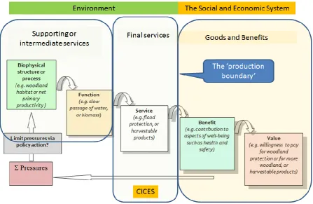
The cascade model from the Common International Classification of Ecosystem Services (CICES) is presented in Figure 2.2 (Haines-Young and Potschin, 2010). The model is designed to unify previous ecosystem service typology systems. CICES incorporates features from the MA, United Kingdom National Ecosystem Assessment (UKNEA) and The Economics of Ecosystems and Biodiversity initiative (TEEB). This provides a platform for ecosystem studies at a range of scales, but adding tiers to the hierarchy, which may blur distinctions between intermediate and final services.

Further, Costanza (2008) suggests that this model still requires adaptation to include issues of scale, ownership and exclusivity. However, the cascade model in Figure 2.2 acts as a useful framework for the ecosystem service approach and as a tool for linking environmental assessment to economic valuations. The titles in the five

cascading boxes follow a gradient from left to right, of factual and easily measureable quantities to subjective, value-led benefits. In particular, there is contention regarding the titles of the third and fourth columns: services and benefits. Costanza et al.,

(29)

[image:29.595.86.534.56.347.2]

8 Figure 2.2. Ecosystem service cascade model (CICES, 2013).

(30)

9 valuations. TEEB acknowledge that cultural and spiritual valuations can be relevant, but they argue that economic valuation should be used as a tool to guide biodiversity management, stating easier interpretation and communication to decision makers (TEEB, 2010). This is further reinforced by Hölzinger et al. (2013) who prepared a comprehensive ecosystem service assessment for Birmingham City Council. Their assessment provided evidence for Birmingham’s Green Living Spaces Plan, which seeks to value Birmingham’s natural resources and features following UKNEA

methodologies. Hölzinger et al. (2013) aimed to calculate the total economic value of as many ecosystem services as possible, citing that rather than being a price-tag for nature, the monetary value is better interpreted as a common denominator for

measurement across ecosystem services. However, they also acknowledge difficulties in providing comparative measurements where economic value is not relevant.

The UKNEA (2011), classify ecosystem services by separating ecosystem processes (underlying ecological functions), intermediate services, and final services - Potschin and Haines-Young’s (2011) ‘benefits’. The UKNEA represents one of the first sub-global assessments after the MA and has been strongly influenced by research commissioned by the Department of Environment, Food and Rural Affairs (DEFRA) (UKNEA, 2011). The UKNEA suggests that the strict economic use of terms such as ‘service’ and ‘goods’ reinforces a bias towards economic measurements and cost-benefit analysis. Conversely, movement away from economics allows more flexibility in classification and definition. Fisher et al., (2009) assert that ecosystem services are “aspects of ecosystems utilised (actively or passively) to produce human well-being” (Fisher et al., 2009, p645). More recently, Bastian et al., (2012, p9) have made this more explicit by defining ecosystem service as “the actually used or demanded contributions made by ecosystems and landscape for human benefit” to distinguish potential capacities from theoretical maxima. These potential services still need to be measured, but measurements can be made up to theoretical maxima. Bastian et al.,

(31)

10 should instead be thought of as environmental settings where physical, social or mental states are changed through the cultural benefits that are consumed or experienced. Much of the debate around these nuances depends on the purpose of study.

2.2.2. Ecosystem service classification systems

Ecosystem service classification provides a structured framework for further scientific analysis (Costanza, 2008). These classification systems have evolved over the years as demonstrated in Figure 2.3.

Building on a list of seventeen services produced by Costanza et al., (1997), subsequent authors have attempted to categorise ecosystem services into distinct classes: the provision of life-sustaining materials, the regulation of the surrounding ecological environment and the requirement for amenable social and psychological experiences with nature. Much research has been conducted into provisioning and regulating services (shaded in orange and green in Figure 2.3), but less has been completed for cultural services, due to challenges finding proxy indicators for measurement and validations (Norton et al., 2012). Habitat services appear in the classifications of de Groot et al., (2002) and TEEB (2010), but do not appear in other classifications. These services are key for consideration of biodiversity and

(32)

(33)

12 Acknowledgement of an inequality in supply and demand across space allows for an amendment to the model produced by Bastian et al., (2012) (Figure 2.4). This allows for a maximum demand or accessibility threshold for service consumption to match the current maximum capacity for service generation, which due to spatial patterns rarely overlaps perfectly. This provides balance to the model produced by Bastian et al., (2012), and emphasises the potential value in approaching ecosystem service research from a value-led direction rather than the more traditional ecosystem property-based measurements. However, Alessa et al., (2008) state that

measurements of demand, usage or value as perceived by humans is societal and subject to change between communities, stakeholders and individuals. This is a challenge when ecosystem services cannot explicitly be measured and boundaries between columns are blurred further (Burkhard et al., 2012). The two ‘potential’

columns provide a relevant, balanced framework for scientific study as data collection and modelling becomes easier when dealing with theoretical capacities than actual human-valued consumption.

Figure 2.4. Revised ecosystem service framework (Author’s own - amended from Bastian et al., 2012).

(34)

13 different ecosystem services. However, there is an emerging consensus, which is reflected in the fact that differences between later evolutions of classification are becoming more subtle (Figure 2.3). Due to its national relevance and holistic approach, the UKNEA ecosystem services framework will be followed within this research. This section has demonstrated that primary data collection remains a challenge as the spatial scales of research often cover wide areas. Consequently, measurements of proxy indicators provide more appropriate assessments of the potential capacities available for consumption. This thesis considers potential

capacities rather than actual generation of ecosystem services as a more appropriate measurement. This provides the maximum levels of generation possible. This

approach allows easier comparison between different cities and regions, and also resolves issues of landscape management and human activity that may differ across space.

2.3. Ecosystem service measurement

The section contains a critical review of different approaches to measure the generation of ecosystem services. The importance of currently neglected spatial analysis is discussed and some of the methodological requirements are revealed (Section 2.3.1). The section closes with a critical review of the current state of multiple ecosystem service generation (Section 2.3.2).

2.3.1. Ecosystem service generation

Ecosystem service assessments measure patterns of generation for specific

ecosystem services or groups of services to determine locations of high ecosystem service generation (known as ecosystem service hotspots) (Egoh et al., 2008);

assess impact of land use; (Koschke et al., 2012) or evaluate how ecosystem service levels change over time (Zhang et al., 2011). This information can inform land

planning decisions based on supply/demand relationships and concepts of

(35)

14 there is sufficient data available to conduct a satisfactory desktop-based urban

ecosystem services assessment, they acknowledge that much baseline data is missing or incomplete. Furthermore, Crossman et al., (2013) state that

inconsistencies in indicator development across the field of research challenge robust valuations and validations of ecosystem services. This makes research difficult to translate across space and through time. Bockstaller and Girardin (2003) stress the importance of developing indicators which meet with scientific standards. This implies a requirement to validate indicators using alternatively collected primary or secondary data (Muller and Burkhard (2012). While this is critical for developing robust methods of ecosystem service assessment, Seppelt et al., (2011) found that a high percentage of studies published include no validation information at all.

Potschin and Haines-Young (2011) suggest that earth surface processes reflect some ecosystem services better than others, which has led to an increase in the analysis of some ecosystem services over others. For example they cite that regulation and provisioning services such as crop production, water flow mitigation and carbon storage generation have been better developed than cultural services such as spirituality or aesthetics, or measurements of service consumption.

Examples of ecosystem service generation mapping include efforts by both Kreuter

et al., (2001) and Liu et al., (2010), which are based exclusively on assigning service generation levels to specific land cover types. Alternatively, Hölzinger et al., (2014) consider the ecosystem services generated by defined habitat types. Frank et al.,

(36)

15 Reginster and Goffette-Nagot (2005) warn that errors in measurement of ecosystem service generation may arise from neglect of neighbouring spaces. For example, Koschke et al., (2012) directly linked ecosystem service provision with CORINE land cover data in Saxony, East Germany and found that this proxy land cover data often does not consider variability within land cover classes or the impacts of different land management. They also discovered that aggregating areas into larger homogenous units exaggerated the influence of urban areas and undermined that of arable farming. Zhang et al., (2011) also cite issues with mismatch in land use composition and heterogeneity and related ecosystem service value estimations. This is

particularly true for cultural services (Plieninger et al., 2013).

Willemen et al., (2014) cite a requirement to improve measures of uncertainty based on simple land cover data. For example, Eigenbrod et al., (2010a) evaluated

generalising errors arising from heterogeneous provision of ecosystem services within single land cover classes. They created three proxy land cover-based service data sets from primary data to explore errors of uniformity, sampling and regionality. They highlight that simple land cover-based mapping of ecosystem services is a poor fit. Chan et al., (2006) corrected for this to an extent by introducing a system of

weighting in their evaluation of ecosystem service generation against biodiversity conservation. However, Koschke et al., (2012) found that weighting services using a prioritisation survey was too challenging for most stakeholders, particularly when asked to rate similar services. Further, many stakeholders did not want to disclose personal demographic information, which meant that analysis of social patterns was frustrated. Consequently, Wu et al., (2013) stress the importance of using appropriate data to build suitable proxies and Rounsevell et al., (2013) highlight the importance of integrating observations and synthetic models. Alternatively, Reginster and Goffette-Nagot (2005) suggest that landscapes have features and processes that have unique spheres of spatial influence with discrete or graduated boundaries signifying

influence thresholds. For example, a football pitch, supplying the environmental settings and opportunity for recreation has defined boundaries, but Bastian et al.,

(2012) note that noise and heat mitigation have blurred boundaries of different sizes.

This section has highlighted the importance of the habitat approach, but has also emphasised the need to build robust indicators that are based on more sophisticated measurements than simple direct relationships with the underlying landscape

(37)

16 ecosystem services can be placed within an Impact component of the Drivers

Pressures State Impact Response (DPSIR) framework. This position is most appropriate because it places ecosystem services between the biophysical measurements of the landscape (State) and the human-well being benefits

generated (Response). Measurement of ecosystem service generation provides a picture of how different ecosystem services are distributed across a landscape. Potschin and Haines-Young, (2013) state that the use of indicators based on landscape features is a common approach because ecosystem service generation can be characterised by biophysical properties. However, the review highlights that indicators of measurement need be more sophisticated than simple land cover maps because ecosystem services are fundamentally related to human activity as well as ecological processes (Muller and Burkhard, 2012). Pleasant et al. (2014) highlight the fact that challenges remain for cultural service measurement due to their non-market value and intangible nature, but frameworks have been altered to allow indicators that incorporate spatial criteria to these services (e.g. UKNEAFO, 2014). For example, by making measurements of environmental settings that provide the potential to produce a service rather than the specific service itself. Crossman et al.

(2014) have also shown that there is demand for better attempts at validation of ecosystem service indicators to provide a measure of confidence that can be used to place research into a more scientific context.

2.3.2. Holistic analysis - multiple ecosystem services

A principal issue in ecosystem service research is the evaluation of relationships between ecosystem services (Rodriguez et al., 2006; Bennett et al., 2009). In their study, Seppelt et al., (2011) note that half of the ecosystem service studies identified, focus on isolated services such as carbon sequestration in urban trees (Davies et al., 2011), or proximity to attractive spaces and amenities (Hamilton and Morgan, 2010). Even the MA assessed its services in isolation (Bennett et al., 2009). There is

growing recognition that ecosystems produce multiple services and ecosystem services are produced by multiple ecosystems (Fisher, et al., 2009; Dobbs et al.,

(38)

17 gardens can all produce food. Brown et al., (2007) suggests that according to the ecosystem approach, these services react and relate to each other and the

landscape from which they are all created. But Gret-Regamey et al., (2014) state that interactions between spatial and temporal scales must be considered to facilitate more relevant ecosystem service generation maps.

Rodriguez et al., (2006) state that ecosystem service relationships can be conflicting or supportive, resulting in service trade-offs or synergies, which are often dynamic over time and space. Bagstad et al. (2013) demonstrate that these relationships depend on how different services exploit required natural resources for generation and also the nature of service consumption by humans. They identify provisioning benefits where the ecosystem service provides the benefit, and preventative benefits, where the ecosystem service mitigates an otherwise harmful process. These require ecosystem services to be modelled in different ways. Alcamo et al. (2005)provide a further example by suggesting that provisioning services are typically destructive in their consumption as they generate products that are eaten as food, or burnt as fuel. Conversely, cultural services may be produced simply by a landscape feature

existing and consumption can potentially be shared with others without diminishing the service for future consumption (Bolund and Hunhammar, 1999).

Bennett et al., (2009) state the importance of ecosystem services that commonly appear together into clusters as a way to consider the relationships between multiple services. This approach emphasises the importance of ecosystem service synergy and promotes the concept of multifunctional landscapes (Plieninger et al., 2013). The majority of research uses ecological units such as land cover or land use (Chan et al., 2006; Nelson et al., 2009; Koschke et al., 2012). However, Raudsepp-Hearne et al., (2010) suggest that the delimitation of clusters into administrative spatial units provides a link to present socio-ecological systems. They claim that use of these administrative units echoes social pressures that influence the flows of ecosystem services. Improvements to this approach could be made by creating bespoke spatial units representing homogenous landscape features, such as Homogenous Urban Patches developed by Herold et al., (2002), which can then be overlaid with existing land use units. This has not yet been done in ecosystem service assessment.

(39)

18 Raudsepp-Hearne et al., (2010) and Ericksen et al., (2012) have both used

ecosystem service clusters to analyse trade-offs between provisioning and regulating services, and provisioning and cultural services. However, both studies use negative correlations of service values across a landscape as evidence of trade-offs. This relationship is not necessarily due to service trade-off, but may be due to different landscape conditions and processes producing different ecosystem services, even standardising trade-off measurements to economic cost simplifies relationships that do not consider underlying drivers of change (Ruiijs et al., 2014). Martin-Lopez et al.,

(2012) derive three distinct ecosystem service clusters: services demanded by urban residents, such as cultural services, air purification and microclimate mitigation, services demanded by rural residents including provisioning services, regulation of soils and water and cultural forestry services, and finally services relating to

agricultural activities. Alternatively, Wu et al., (2013) found trade-offs across North East China, between a natural service cluster composed of soil retention, habitat services and carbon sequestration, and an artificial service cluster composed of material production and population support. However, their choice of ecosystem services highlights the issue of typological inconsistency across the discipline. On the other hand, Van der Biest et al., (2014) applied a Bayesian belief approach to

develop an ecosystem service cluster index incorporating biophysical and socio-economic properties. Based on these inputs and current land use patterns, the index was calculated with current land use patterns and optimal land use patterns to

determine a value of difference indicating potential for improvement. However, they cite weighting in the belief network and validation as issues to be overcome.

To operationalise the ecosystem approach, the UKNEAFO (2014) have developed a suite of tools for use by decision makers (Scott et al., 2014). These tools serve to assist in matters of planning regulation, land management incentives, engagement with local communities, valuations and trade-offs, and future predictions of

(40)

19 developed at national scales, such as the INtegrated Valuation of Ecosystem

Services and trade-offs (INVEST) and the Artificial Intelligence for Ecosystem Services (ARIES). These models are now commonly used in research studies to value ecosystem services at a national level (e.g. Nelson et al., 2009; Villa et al.,

2009; Kareiva et al., 2011). These models are highly sophisticated, but often require significant levels of expertise, data acquisition and processing times. Further,

Vigerstol and Aukema (2011) note that fundamental mechanisms behind the programmes are different: INVEST is deterministic and based on simplifications of current models, while ARIES is based on probabilistic models. This means that inputting the same variables into these models is likely to produce different results and to-date, no comparison or verification has been made between them. Computer models have also started to incorporate 3D elements, although generally only for visual purposes so far (Gret-Regamey et al., 2013). This review section highlights the requirement to develop the integration of 3D data into ecosystem service models as an approach to improve mapping and produce new questions on the impact that the 3D urban form may have on ecosystem service distribution, connectivity and flow.

Potschin and Haines Young (2013) recommend a place-based approach to

perceiving the ecosystem service framework, which considers how different clusters of ecosystem services have different social values dependent on their location. This approach as applied by Sherouse et al., (2011) involves a focus on participatory data collection and engagement with local communities to discern how services and clusters are differently viewed. Raymond et al., (2009) suggest that this is potentially the most important for determining perceptions of ecosystem service values and indeed may be the only method of truly capturing cultural service valuations at the local scale as it engages with local communities. But, a major drawback of the place-based approach is the lack of transferability, even to alternative locations very close by (Alessa et al., 2008). As each research site is unique, so too are the values placed on service clusters. This raises questions about the feasibility of generating

ecosystem service indicators that satisfy the place-based approach.

This review section has highlighted the requirement to improve on clustering of multiple ecosystem services over space (Raudsepp-Hearne et al. 2010).

(41)

20 that producing bespoke spatial units may improve characterisation of ecosystem service generation patterns over a city to better manage and maintain acceptable levels (Potschin and Haines-Young, 2013). GIS and remote sensing technologies have proven to be a useful platform for such research (Jackson et al., 2013). However, there is a demand for models that can accurately reflect patterns of ecosystem service generation across a diverse urban landscape (Bagstad et al.,

2013). The next section considers the left-hand side of Figure 2.1 and Figure 2.3, which focus on how accessibility to services can be used as a measurement of potential ecosystem service consumption.

2.4. Ecosystem service accessibility

2.4.1. Ecosystem service accessibility as a measure of ecosystem service consumption

Ecosystem service consumption is less well understood than ecosystem service generation (Bastian et al 2012). This is because it is more challenging to measure as it deals with human values rather than objective measurements. Ecosystem service consumption occupies the right hand side of Haines-Young and Potschin’s cascade model in Figure 2.1 (CICES, 2013). The review in this section evaluates the

application of accessibility to ecosystem services as a proxy for potential ecosystem service consumption. Physical accessibility and observer visibility studies are

evaluated for their potential to provide different perspectives and raise new questions on ecosystem service consumption.

Valuation of ecosystem services is a key outcome of many ecosystem service assessments. This determines the level of demand and provides justification for management actions (Boyd and Banzhaf, 2007; TEEB, 2010). Economic

measurements are the most common, based on cost per unit. These provide simple comparative results for non-specialist decision makers (Brown et al., 2007). However, Sagoff (2011) criticises these methods as being blunt and simplistic. Liu et al., (2010) and Brown et al., (2007) continue, stating that different valuations arise from dynamic market conditions and economic data quality and coverage. Sherrouse et al., (2011) suggest that economic measurements ignore relationships between people and place, where bequest or existence values may be valued more highly. These focus on experiential cultural services and less tangible regulatory services that are

(42)

21 and adds a dimension that cannot be collected through analysis of land cover

mapping, making quantification and generalisations challenging (Vizzari, 2011). Moreover, local knowledge is often incomplete, only focussing on issues of subjective importance to local stakeholders, potentially neglecting influential underlying issues (Raymond et al., 2009). There is a drive towards developing non-monetary

quantification based on physical service units (Boyd and Banzhaf, 2007; Burkhard et al., 2012).

A solution to this presents itself through analysis of accessibility to ecosystem services. Schroter et al., (2014) suggest that access to greenspaces provides the opportunity for humans to consume or experience the services and benefits produced by in an ecosystem. Without this mechanism, there are no ecosystem services as there no stakeholders to benefit (Burkhard et al., 2012). Hedonic pricing analysis has emerged as a common method of determining access to ecosystem services, relating the Euclidean proximity of amenities and attractions (ecosystem services) to house prices (Wu et al., 2004; Ready and Abdaller, 2005; Sander and Polasky, 2009). Sander and Haight (2012) consider hedonic pricing analysis of cultural ecosystem services in relation to property prices in Dakota County, USA. They found that access to recreational spaces and the proximity of trees increased prices, but they only considered Euclidean distances. Kovacs (2012) also

emphasises the importance of the ecosystem service clusters in urban parks on property prices. He suggests that the optimum percentage of parkland within a half mile neighbourhood around a property is 20%, although he also find that homes in immediate proximity to parks have lower values, due to higher levels of noise and a higher risk of crime. Klaiber and Phaneuf (2010) state that the quality of parks may reduce house prices if they are not maintained. While this work focuses on economic valuation in relation to open space proximity, accessibility is also linked to health. Reyes et al., (2014) find that accessibility to parks is higher in suburban areas and generally supports previous theories that lower socio-economic classes have lower access and are affected adversely as a result (Lucas and Jones, 2012). That said, Witten et al., (2008) and Timperio et al., (2007) found no relationships between park access and socio-economic status, while Cradock et al., (2005) and Ellaway et al.,