http://dx.doi.org/10.4236/am.2014.519290
How to cite this paper: Clementi, S., Fernandi, M., Decastri, D. and Bazzurri, M. (2014) Mixture Optimization by the CARSO Procedure and DCM Strategies. Applied Mathematics, 5, 3026-3039. http://dx.doi.org/10.4236/am.2014.519290
Mixture Optimization by the CARSO
Procedure and DCM Strategies
Sergio Clementi
1,2*, Mauro Fernandi
3, Diego Decastri
3, Matteo Bazzurri
11Chemistry Department, University of Perugia, Perugia, Italy 2M.I.A. Multivariate Infometric Analysis Srl, Perugia, Italy 3Flint Group Italia, Cinisello Balsamo, Milano, Italy Email: *[email protected]
Received 29 August 2014; revised 25 September 2014; accepted 12 October 2014
Copyright © 2014 by authors and Scientific Research Publishing Inc.
This work is licensed under the Creative Commons Attribution International License (CC BY). http://creativecommons.org/licenses/by/4.0/
Abstract
The paper illustrates a new way of using the CARSO procedure for response surfaces analyses de-rived from innovative experimental designs in multivariate spaces, based on Double Circulant Matrices (DCMs). We report a case study regarding a design based on a DCM for 4 variables. The final response surface model is obtained by the formerly developed CARSO method.
Keywords
CARSO Procedure, Design Strategies, Circulant Matrices (DCM), Optimization
1. Introduction
Following our previous paper published on November 2012 [1], where we showed a strategy for collecting the data needed for defining a response surface on the basis of a D-optimal design, we present now a further innova-tive strategy that requires a much lower number of experimental data, based on Double Circulant Matrices (DCMs). In fact chemical processes involve products which are mixtures of several components, and the objec-tive of industrial research is reaching the best level of technological properties the mixture is expected to exhibit. The way mixtures are produced today is often based on established knowledge and tradition rather than on a scientific approach by statistical or chemometric strategies.
ate response surfaces. The final response surface model is obtained by the formerly developed CARSO method [5], where the surface equation is derived by a PLS model on the expanded matrix, containing linear, squared and bifactorial terms, and studied at extreme points by Lagrange analysis.
2. Central Composite Design
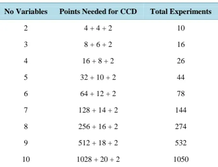
[image:2.595.185.411.247.420.2]This strategy requires that all planned experiments should contain all mixture constituents, in such a way that we use the lowest number of points, so that the design is centrosymmetrical, i.e. distributed in a well balanced way within the multivariate space (all experimental points have the same distance from the origin), with the addition of a few experiments (almost two) at the central point. The CCD strategy can be used profitably only with two or three variables, otherwise it requires too many experiments, as shown in the following Table 1[10].
Table 1. Number of experiments needed for a CCD for each number of variables.
No Variables Points Needed for CCD Total Experiments
2 4 + 4 + 2 10
3 8 + 6 + 2 16
4 16 + 8 + 2 26
5 32 + 10 + 2 44
6 64 + 12 + 2 78
7 128 + 14 + 2 144
8 256 + 16 + 2 274
9 512 + 18 + 2 532
10 1028 + 20 + 2 1050
3. Double Circulant Matrices (DCMs)
Our main objective of our industrial research was finding out methods of collecting data with the lowest possible number of experiments, but still keeping the roundness of the experimental design, focused on the CCD strategy. Because of this we wanted to test the efficacy of double circulant matrices. Starting from the knowledge of how to manage a Central Composite Design, where the levels of each variable are settled according to the increasing coded values in the experimental space, we tried to build the second half of the experimental coded matrix just changing the order of the values with respect to the first half. Indeed we had good and sound results to build a response surface, and therefore we could obtain the experimental conditions to optimize the property of the mixture, using a much smaller number of experiments (Table 2) [10]. The DCMs have quite a number of prop-erties that make them to be very efficient for experimental design. In particular they still have a roundness equal to CCD, but they require a much smaller number of experiments. We present here (Table 3) the simplest case study, with four variables, coupling submatrices (briefly sm) sm1 and sm3.
In order to simplify the comprehension of a DCM we wish to observe that each DCM contains three blocks of rows: 1) the circulant sm generated by the fundamental permutation, i.e. the sequence of coded values increasing from −1 to 1, according to the squared spacing; 2) a second circulant sm generated by one of the other permuta-tions possible, in such a way to be the most different (the most orthogonal) from the fundamental one; 3) a group (at least two objects) with all variables equal to zero to represent the central point of the experimental work.
3.1. Selection of Coded Values
Table 2. Experiments needed for CCD and DCM for each number of variables.
No Variables Experiments for CCD Experiments for DCM
2 10 -
3 16 -
4 26 10
5 44 12
6 78 14
7 144 16
8 274 18
9 532 20
[image:3.595.184.410.318.507.2]10 1050 22
Table 3.DCM4: 4 variables, 4 levels, 10 experiments―spac- ing function of squares.
VAR 1 VAR 2 VAR 3 VAR 4
EXP.1 −1 −0.58 0.58 1
EXP.2 −0.58 0.58 1 −1
EXP.3 0.58 1 −1 −0.58
EXP.4 1 −1 −0.58 0.58
EXP.5 −0.58 1 0.58 −1
EXP.6 1 0.58 −1 −0.58
EXP.7 0.58 −1 −0.58 1
EXP.8 −1 −0.58 1 0.58
EXP.9 0 0 0 0
EXP.10 0 0 0 0
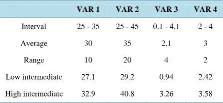
case, the total variation (2) should be divided by 3, obtaining 0.67, so that the first interval ranges from −1 to −0.33, the second ranges from −0.33 to 0.33, and the third ranges from 0.33 to 1. However, since we need to mimic the CCD, the distance should be computed in the space of the squares, instead of using the linear distance. The square root of 0.33 is 0.58: therefore the intermediate levels are −0.58 and 0.58. We show the real case study for a better understanding of the procedure (Table 4) that gives the subsequent experimental design (Table 5):
Table 4. DCM4: Computation of real values for coded values.
VAR 1 VAR 2 VAR 3 VAR 4
Interval 25 - 35 25 - 45 0.1 - 4.1 2 - 4
Average 30 35 2.1 3
Range 10 20 4 2
Low intermediate 27.1 29.2 0.94 2.42
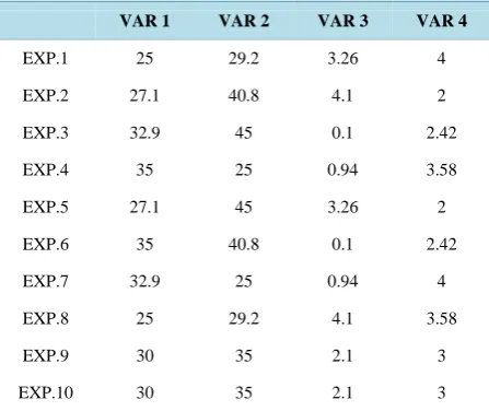
[image:3.595.185.409.617.721.2]Table 5. DCM4: experimental design.
VAR 1 VAR 2 VAR 3 VAR 4
EXP.1 25 29.2 3.26 4
EXP.2 27.1 40.8 4.1 2
EXP.3 32.9 45 0.1 2.42
EXP.4 35 25 0.94 3.58
EXP.5 27.1 45 3.26 2
EXP.6 35 40.8 0.1 2.42
EXP.7 32.9 25 0.94 4
EXP.8 25 29.2 4.1 3.58
EXP.9 30 35 2.1 3
EXP.10 30 35 2.1 3
3.2. Characteristics of DCMs
The Double Circulant Matrices show some peculiar characteristics. First of all the rank of the experimental ma-trix is (n − 1) since each row sums up to 0 using coded values. At the same time also each column sums up to 0 using coded values. As a consequence these “objects” are very extreme in terms of internal symmetry. The first row of the first half of a DCM is always written reporting the increasing coded values for the sequence of va-riables. Then, the following rows are written shifting on the left the coded values and putting in the last column the term sitting in the first one in the previous row, until all values have been located in all columns. The second half of the matrix requires a different order of the coded values and this opens a new problem.
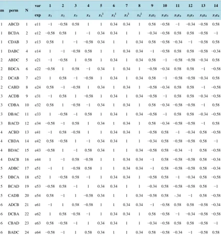
The number of possible permutations of the order of coded values is n! This means that the total permutations for a DCM4 are 24, divided into six groups of 4 rows A strategy is needed for selecting the “best” sm to be coupled with the obvious first half. The main objectives are twofold: finding out the two sm.s less correlated, and avoiding that the two sm.s have identical columns, thus showing no variance in the eight remaining rows.
3.3. Selection of the Submatrices to Be Tested
At first we started to study the characteristics of each sm in terms of the volume occupied with respect to that of the full matrix, but we soon realized that this approach could be not enough reliable, beside being impossible to handle on increasing the number of variables. Meanwhile, we paid attention to the presence of the same coded values for some of the variables, namely the bifactorial terms. Indeed already the generating sm (sm1) has two identical columns (variable 10: x1x3 and 13: x2x4) with all values set at −0.58. This means that it is not possible to
use together sm1 and sm6, because they would have two constant variables. For an almost similar reason sm1 should not be coupled with sm4 and sm5, which have always the same variables set at 0.58, so that these col-umns would have only two levels. Therefore the choice is restricted to the couples (sm1 + sm2) or (sm1 + sm3). The complete list of all the 24 permutations for the four variable case is reported in Table 6. The coded values are A = −1, B = −0.58, C = 0.58, D = 1.
Since this case is the easiest for the DCMs we decided to make an experimental test using all the first three sm.s, in order to verify which couple could give better predictions on the objects of the left out sm. The results, reported in the experimental part, clearly showed that the couple (sm1 + sm3) gave better predictions for the ob-jects of sm2 with respect to the model (sm1 + sm2) projected on the obob-jects of sm3.
Table 6. List of the expanded permutations for a DCM4.
sm perm N
var 1 2 3 4 5 6 7 8 9 10 11 12 13 14
exp x1 x2 x3 x4 x12 x22 x32 x42 x1x2 x1x3 x1x4 x2x3 x2x4 x3x4
1 ABCD 1 e11 −1 −0.58 0.58 1 1 0.34 0.34 1 0.58 −0.58 −1 −0.34 −0.58 0.58
1 BCDA 2 e12 −0.58 0.58 1 −1 0.34 0.34 1 1 −0.34 −0.58 0.58 0.58 −0.58 −1
1 CDAB 3 e13 0.58 1 −1 −0.58 0.34 1 1 0.34 0.58 −0.58 −0.34 −1 −0.58 0.58
1 DABC 4 e14 1 −1 −0.58 0.58 1 1 0.34 0.34 −1 −0.58 0.58 0.58 −0.58 −0.34
2 ABDC 5 e21 −1 −0.58 1 0.58 1 0.34 1 0.34 0.58 −1 −0.58 −0.58 −0.34 0.58
2 BDCA 6 e22 −0.58 1 0.58 −1 0.34 1 0.34 1 −0.58 −0.34 0.58 0.58 −1 −0.58
2 DCAB 7 e23 1 0.58 −1 −0.58 1 0.34 1 0.34 0.58 −1 −0.58 −0.58 −0.34 0.58
2 CABD 8 e24 0.58 −1 −0.58 1 0.34 1 0.34 1 −0.58 −0.34 0.58 0.58 −1 −0.58
3 ACDB 9 e31 −1 0.58 1 −0.58 1 0.34 1 0.34 −0.58 −1 0.58 0.58 −0.34 −0.58
3 CDBA 10 e32 0.58 1 −0.58 −1 0.34 1 0.34 1 0.58 −0.34 −0.58 −0.58 −1 0.58
3 DBAC 11 e33 1 −0.58 −1 0.58 1 0.34 1 0.34 −0.58 −1 0.58 0.58 −0.34 −0.58
3 BACD 12 e34 −0.58 −1 0.58 1 0.34 1 0.34 1 0.58 −0.34 −0.58 −0.58 −1 0.58
4 ACBD 13 e41 −1 0.58 −0.58 1 1 0.34 0.34 1 −0.58 0.58 −1 −0.34 0.58 −0.58
4 CBDA 14 e42 0.58 −0.58 1 −1 0.34 0.34 1 1 −0.34 0.58 −0.58 −0.58 0.58 −1
4 BDAC 15 e43 −0.58 1 −1 0.58 0.34 1 1 0.34 −0.58 0.58 −0.34 −1 0.58 −0.58
4 DACB 16 e44 1 −1 0.58 −0.58 1 1 0.34 0.34 −1 0.58 −0.58 −0.58 0.58 −0.34
5 ADBC 17 e51 −1 1 −0.58 0.58 1 1 0.34 0.34 −1 0.58 −0.58 −0.58 0.58 −0.34
5 DBCA 18 e52 1 −0.58 0.58 −1 1 0.34 0.34 1 −0.58 0.58 −1 −0.34 0.58 −0.58
5 BCAD 19 e53 −0.58 0.58 −1 1 0.34 0.34 1 1 −0.34 0.58 −0.58 −0.58 0.58 −1
5 CADB 20 e54 0.58 −1 1 −0.58 0.34 1 1 0.34 −0.58 0.58 -.34 −1 0.58 −0.58
6 ADCB 21 e61 −1 1 0.58 −0.58 1 1 0.34 0.34 −1 −0.58 0.58 0.58 −0.58 −0.34
6 DCBA 22 e62 1 0.58 −0.58 −1 1 0.34 0.34 1 0.58 −0.58 −1 −0.34 −0.58 −0.58
6 CBAD 23 e63 0.58 −0.58 −1 1 0.34 0.34 1 1 −0.34 −0.58 0.58 0.58 −0.58 −1
6 BADC 24 e64 −0.58 −1 1 0.58 0.34 1 1 0.34 0.58 −0.58 −0.34 −1 −0.58 0.58
Because of this we repeated the computation on excluding the squared terms (they are needed for building the model of the response surface, but, since they are all positive, their presence may be dangerous, and therefore they should be excluded for computing vector angles). Indeed, on computing the angles between vectors with 40 elements non scaled, the results indicate a cosine zero for the couples (sm1 + sm3) and (sm1 + sm5), but the second choice, as stated earlier, involves two columns with only two coded values, and therefore should be dis-regarded.
4. Case Study (Experimental Part)
We should first state that, because of the high internal symmetry of DCMs, but mainly because of the steps se-quence needed in the optimization study (1) perform the experimental design, 2) compute the response surface, 3) select and measure a few new appealing mixtures, and 4.adding their results to the first design, in order to get a refined model), the ordinary CARSO procedure must be slightly modified. Indeed, the first module of the pro-gram CARSO (CODER) expands the matrix scaling all variables between 1 and −1. On using DCMs we feel that it is much better to work with non-scaled data (that keeps all the roundness), and therefore the expanded matrix should be analyzed without autoscaling. In fact, on adding the new mixtures to the experimental design (often outside of its domain) the model changes significantly and therefore it is difficult to understand, while it is much simpler to align the new objects to the coding of the design.
[image:6.595.87.539.337.635.2]The case study regards the optimization of the technological properties of an ink containing four ingredients (variables). The properties are contact angle (CA, the most important, to be minimized), blocking resistance (BR, also important to be maximized), and adhesion (AD, to be minimized). It is also noteworthy to remind that the response surface is aimed to find out the highest values of the y. Therefore, for properties to be minimized, the response must be expressed as its inverse, i.e. 1/y. As stated previously, we started our collection of data on tak-ing into account all the mixtures belongtak-ing to sm1, sm2 and sm3, i.e. objects from 1 to 12 of Table 6; obviously, the real data used are those shown in Table 5. The measurements of the three technological properties are listed in Table 7. The contact angle is measured by a CAM200 contact angle meter (KSV), while the other two prop-erties are evaluated by ordinal data. Because of this also adhesion should be maximized.
Table 7. Experimental design and technological properties.
N EXP x1 x2 x3 x4 1/CA 1/CAc BR BRc AD ADc
1 e11 −1 −0.58 0.58 1 8.13 0 5 100 3 50
2 e12 −0.58 0.58 1 −1 13.12 93.4 2 25 5 100
3 e13 0.58 1 −1 −0.58 8.46 6.2 5 100 4 75
4 e14 1 −1 −0.58 0.58 8.98 15.8 4.5 87.5 1 0
5 e21 −1 −0.58 1 0.58 8.45 6 5 100 4 75
6 e22 −0.58 1 0.58 −1 13.48 100 2 0.25 5 100
7 e23 1 0.58 −1 −0.58 8.96 15.5 5 100 4 75
8 e24 0.58 −1 −0.58 1 8.24 2.1 5 100 1 0
9 e31 −1 0.58 1 −0.58 12.85 88.3 3 50 5 100
10 e32 0.58 1 −0.58 −1 10.52 44.6 3.5 62.5 5 100
11 e33 1 −0.58 −1 0.58 8.15 0.4 5 100 1 0
12 e34 −0.58 −1 0.58 1 8.35 4.1 5 100 2 25
13 cc1 0 0 0 0 8.33 3.7 5 100 3 50
14 cc2 0 0 0 0 8.41 5.2 5 100 3 50
On inspecting the trends of the y values it is immediately clear that contact angle and blocking show an oppo-site effect on changing the relative amounts of the variables, while contact angle and adhesion are somewhat correlated. Therefore the main objective of this study is to find the best compromise between the y variables.
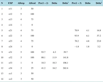
Table 8. Comparison of goodness of predictions for blocking resistance. The SDEP values are 12.4 for (sm1 + sm2) and 5.9 for (sm1 + sm3).
N EXP BRexp BRcod Pre(1 + 2) Delta Delta2 Pre(1 + 3) Delta Delta2
1 e11 5 100
2 e12 2 25
3 e13 5 100
4 e14 4.5 87.5
5 e21 5 100 91.3 8.7 75.69
6 e22 2 25 29.8 4.8 23.04
7 e23 5 100 95.6 4.4 19.36
8 e24 5 100 95.2 4.8 23.04
9 e31 3 50 34.5 15.5 240.3
10 e32 3.5 62.5 80.0 17.5 306.3
11 e33 5 100 99.0 1.0 1.0
12 e34 5 100 108.4 8.4 70.8
13 cc1 5 100
14 cc2 5 100
Table 9. Comparison of goodness of predictions for adhesion. The SDEP values are 11.7 for (sm1 + sm2) and 4.5 for (sm1 + sm3).
N EXP ADexp ADcod Pre(1 + 2) Delta Delta2 Pre(1 + 3) Delta Delta2
1 e11 3 50
2 e12 5 100
3 e13 4 75
4 e14 1 0
5 e21 4 75 70.9 4.1 16.8
6 e22 5 100 93.9 6.1 37.2
7 e23 4 75 70.2 4.8 23.0
8 e24 1 0 −1.8 1.8 3.2
9 e31 5 100 93.7 6.3 39.7
10 e32 5 100 88.1 11.9 141.8
11 e33 1 0 10.3 10.3 106.1
12 e34 2 25 41.2 16.2 262.4
13 cc1 3 50
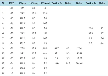
[image:7.595.118.477.435.719.2]Table 10. Comparison of goodness of predictions for the inverse of contact angles. The SDEP values are 8.9 for (sm1 + sm2) and 8.2 for (sm1 + sm3).
N EXP CAexp 1/CAexp 1/CAcod Pre(1 + 2) Delta Delta2 Pre(1 + 3) Delta
1 e11 123 8.1 0
2 e12 76.2 13.1 92.6
3 e13 118.2 8.5 7.4
4 e14 111.4 9.0 16.7
5 e21 118.3 8.5 7.4 20.4 13
6 e22 74.2 13.5 100 93.3 6.7
7 e23 111.6 9.0 16.7 9.1 7.6
8 e24 121.3 8.2 1.9 2.3 0.4
9 e31 77.8 12.9 88.9 84.7 4.2 17.6
10 e32 95.1 10.5 44.4 35.1 9.3 86.49
11 e33 122.7 8.2 1.9 5.4 3.5 12.25
12 e34 119.8 8.4 5.2 -9.0 14.2 201.64
13 cc1 120.1 8.3 3.7
14 cc2 118.9 8.4 5.2
4.1. Selection of the Best Couple of Submatrices
The results illustrated in the previous section clearly showed that, for all the three technological properties in-vestigated, the model derived by the couple (sm1 + sm3) always gives better predictions for the left out objects of sm2, with respect to the model derived by the couple (sm1 + sm2) that gives worse predictions for the left out objects of sm3. Consequently, we proved experimentally that, for DCM4, the best choice is to couple sm3 to the fundamental sm1, since we already stated in Section 3.3 that sm6 would give a system with two identical col-umns, whereas sm4 and sm5 would give a system with the same two columns with only two coded values.
4.2. Optimization Study
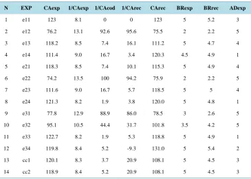
The second part of our study is aimed to perform an optimization study, by obtaining, for each of the three tech-nological properties, a response surface model on using the PLS algorithm on the expanded matrix (containing linear, squared and bifactorial terms, as shown in Table 6, taking into account the objects 1 - 12 plus the two central points). Indeed, even if we demonstrated which of the two couples shows better predictions, once we collected the experimental data on all the three submatrices, it seems appropriate to use all of them for obtaining more stable results for the problem under investigation. The optimization study by computing the response sur-faces has been derived from the data in Table 7 and gave the results listed in Table 11.
The software used is CARSO [5], modified as stated at the beginning of Section 4, and the final goal is to find the best compromise between the three properties both on computing, from the single y values, a total desirabil-ity function, and evaluating if the prediction value of each property reaches the desired measures.
Furthermore, even if we demonstrated that a two latent variables model generates better predictions with re-spect to a single latent variable, we preferred to use for our work only the first one for the following reasons. On one side the first latent variable explains already a very high percentage of the y variation (88% for 1/CA, 82% for BR and 95% for AD), but the straight line of the model is constrained to fit a few good or bad points (usually one for each submatrix) to all the others.
Table 11. Technological values recomputed for each object and property.
N EXP CAexp 1/CAexp 1/CAcod 1/CArec CArec BRexp BRrec ADexp
1 e11 123 8.1 0 0 123 5 5.2 3
2 e12 76.2 13.1 92.6 95.6 75.5 2 2.2 5
3 e13 118.2 8.5 7.4 16.1 111.2 5 4.7 4
4 e14 111.4 9.0 16.7 3.4 120.3 4.5 4.9 1
5 e21 118.3 8.5 7.4 10.1 115.3 5 4.9 4
6 e22 74.2 13.5 100 94.2 75.9 2 2.2 5
7 e23 111.6 9.0 16.7 5.7 118.5 5 5 4
8 e24 121.3 8.2 1.9 3.8 120.0 5 4.8 1
9 e31 77.8 12.9 88.9 86.0 78.5 3 2.6 5
10 e32 95.1 10.5 44.4 31.7 101.8 3.5 4.2 5
11 e33 122.7 8.2 1.9 5.3 118.8 5 4.9 1
12 e34 119.8 8.4 5.2 -9.3 131.0 5 5.4 2
13 cc1 120.1 8.3 3.7 20.9 108.1 5 4.5 3
14 cc2 118.9 8.4 5.2 20.9 108.1 5 4.5 3
4.3. Relationships between the Technological Properties
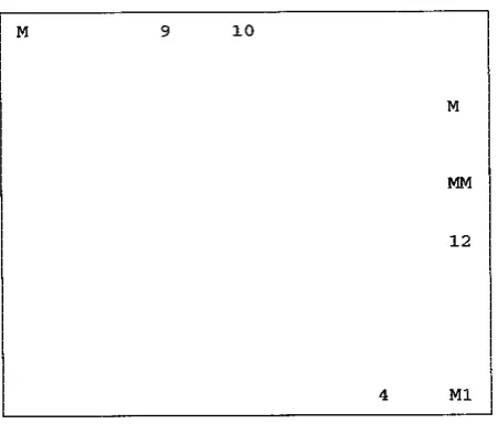
The relationships between the three technological properties are shown in Figures 1-3. Figure 1 depicts the trends between contact angle (CA) and blocking resistance (BR), which appears to be almost a perfect line if we accept that the points 7 and 9 could have had an ordinal value half point higher than the true one. Anyway the relationship shows that on increasing CA (thus moving to worse values) we find high values (best results) for BR. Figure 2 illustrates the behaviour between contact angle (CA) and adhesion (AD), that shows a somewhat peculiar trend. Clearly the four objects (2, 6, 9 and 10) with the best values for CA are the same for the best ob- jects for AD, which at first gave the impression that these two properties were highly correlated. Indeed, for high values of CA, AD shows both good and bad values. This is also confirmed by Figure 3 (BR vs. AD) which shows even better this peculiarity of AD.
[image:9.595.186.411.506.693.2]Figure 2. Plot of contact angle vs. adhesion for experimental points.
Figure 3. Plot of blocking resistance vs. adhesion for experi-mental points.
4.4. New Predictions
On the basis of the three response surfaces found, that always show a maximum within the coded limits of va-riables, but with y variables higher than the data collected in the experimentation, which indicate a hyperbell with a maximum inside the limits of the x variables, the first mixtures to be checked are the mixtures at the ver-tices of the cube of our experimentation. The predictions for these points are listed in Table 12.
4.5. Study of the Coefficients of the Quadratic Equation
The study of the coefficients of the quadratic equation gives the results listed on the left of Table 13 without the correction for the different ranges of each term (see Table 6: the linear terms have a range of 2, the quadratic terms have a range of 0.66 and the bifactorial terms have a range of 1.58), whereas those on the right have been computed by using this correction.
In both cases the coefficients for x1 and x4 are negative for 1/CA and for AD, while the coefficients for x2 and
x3 are positive, but the coefficients for BR have an opposite sign. This result clearly shows that the optimization
[image:10.595.182.412.87.273.2] [image:10.595.186.412.308.500.2]Table 12. Predictions on the vertices of the experimental domain.
N EXP x1 x2 x3 x4 CApre BRpre ADpre
1 V1 1 1 1 1 105.8 4.4 2.3
2 V2 1 1 1 −1 84.7 3 4.6
3 V3 1 1 −1 1 117.9 4.9 3.3
4 V4 1 −1 1 1 125.7 5 2.6
5 V5 −1 1 1 1 96.4 3.9 4.1
6 V6 1 1 −1 −1 114.5 4.8 5.7
7 V7 1 −1 1 −1 102.8 4.2 2.4
8 V8 −1 1 1 −1 69 1.5 6
9 V9 1 −1 −1 1 78.5 2.6 3.1
10 V10 −1 1 −1 1 108.9 4.5 2.5
11 V11 −1 −1 1 1 133.5 5 4.8
12 V12 1 −1 −1 −1 119.5 5 3
13 V13 −1 1 −1 −1 89.3 3.4 4.5
14 V14 −1 −1 1 −1 90.6 3.5 4.3
15 V15 −1 −1 −1 1 124.8 5 2.8
16 V16 −1 −1 −1 −1 105.8 4.4 2.3
Table 13. Relative importance of each variable for each property.
1/CA BR AD 1/CA BR AD
1 LV 1 LV 1 LV 1 LV 1 LV 1 LV
var 89% 82% 97% 89% 82% 97%
x1 −0.29 0.24 −0.26 −0.09 0.08 −0.1
x2 0.41 −0.4 0.61 0.15 −0.15 0.23
x3 0.42 −0.4 0.29 0.14 −0.13 0.09
x4 −0.51 0.54 −0.6 −0.19 0.2 −0.22
which one should be privileged. In principle the most important property is the contact angle (as low as possible), provided that the blocking resistance is good enough (with an ordinal value of at least 3.5).
In particular this table shows that on increasing x1 and x4 and decreasing x2 and x3 we can obtain better values
for CA and AD, but a worse value for BR, while on decreasing x1 and x4 and increasing x2 and x3 we can obtain
better values for BR, but worse values for CA and AD.
4.6. Further Predictions
On the basis of these observations we computed the predictions of a few further mixtures within and just outside the experimental design (we wish to remind that predictions on points outside the domain should have a de-creasing reliability on inde-creasing the distance from the design borders), with the objective to find out a reasona-ble compromise between the behaviours of CA and AD versus BR, which shows an opposite trend. The predic-tions for these points are listed in Table 14.
Table 14. Further predictions within and just outside the experimental domain.
N EXP x1 x2 x3 x4 CApre BRpre ADpre
1 p1 0 1 1 −1 75.8 2.2 4.7
2 p2 0 1 1 0 88.2 3.3 2.9
3 p3 0 1 0 0 98.8 4 2.1
4 p4 −1 1.5 1.5 −1 60.4 0 8.5
5 p5 −1.2 1.2 1.2 −1.2 62.1 0 7.8
6 p6 −0.8 0.8 0.8 −0.8 76.6 2.3 4.4
7 p7 −0.7 0.7 0.7 −0.7 80.5 2.7 3.7
8 p8 −0.6 0.6 0.6 −0.6 84.5 3 3.1
9 p9 −0.5 0.5 0.5 −0.5 88.6 3.4 2.6
10 p10 −0.7 0.5 0.7 0 90.1 3.5 2.6
can either select a mixture that gives a good CA but BR is much lower than the agreed level (p1 or p9), or a mixture that reaches the agreed level of BR but with CA in the range of 90 (p10). The peculiar behaviour of ad-hesion does not help, because for the only point (p10) that satisfy BR adad-hesion reaches a much too low ordinal value. Consequently the company has decided to repeat the same type of study using five different ingredients. This new study has indeed given the expected results, that we shall report in a next paper.
5. Conclusions and Perspectives
Although the results of this first study based on collecting data on a DCM could not yet be used by the company for improving the quality of its products, the experience gained in this work will be helpful for testing what will happen with larger matrices.
In particular we have clearly seen, just because we used all three sm.s, that each sm contains only one mixture giving good results, a second mixture with more or less fairly good ones, while the other two mixtures give low results. This result is not surprising: on the contrary it was somewhat expected, because each sm covers the 4D space in a regular circulant way, that creates a similar relative distance between objects, even if in different sec-tors of the hyperspace. If this will be proven to be true also for larger matrices, as we expect, the problem of se-lecting the best couple (by measuring the cosines of vector angles or by orthogonality criteria) might be aban-doned, just because each sm to be added to the generating sequence (from the lower to the higher coded value) can bring always the same type of global information.
Consequently the perspectives for the next study by a DCM5 on a new formula probably will not be ad-dressed to the objectives just discussed, but only taking care of checking the absence of the risk of having in the bifactorial terms columns with only the same figures or just two values. In principle this risk should diminish on increasing the number of variables, but we shall face the problem of the difference between cases with an even number of variables and cases with an odd number of variables. Indeed, in the second case, the coded value of the central point is zero, and this means that it will be impossible to avoid equal values in a column, because the linear, the quadratic and all bifactorial terms involving this code will be zero. All the results regarding this new case will be reported in our next paper. However, in order to clarify our conclusions we add two more sections, on the relative predictions with two or three sm.s, and on the comparison between DCM and CCD.
5.1. Comparison of Predictions with 2 and 3 sm
Table 15. Comparison of predictions with (s1 + s2), (s1 + s3) and the full model (s1 + s2 + s3).
N EXP x1 x2 x3 x4 CA123 CA12 CA13 BR123 BR12 BR13 AD123 AD12 AD13
1 p1 0 1 1 −1 75.8 75.7 78.2 2.2 2.1 2.5 4.7 5 5.4
2 p2 0 1 1 0 88.2 90.1 89.8 3.3 3.4 3.5 2.9 4.3 4.4
3 p3 0 1 0 0 98.8 101.1 103 4 4.1 4.2 2.1 3.8 3.9
4 p4 −1 1.5 1.5 −1 60.4 60.4 61.4 0 0 0.6 8.5 5.4 5.9
5 p5 −1.2 1.2 1.2 −1.2 62.1 62.3 63.1 0 0.3 0.9 7.8 5.3 5.7
6 p6 −0.8 0.8 0.8 −0.8 76.6 77.8 78 2.3 2.3 2.5 4.4 4.7 4.9
7 p7 −0.7 0.7 0.7 −0.7 80.5 82 82.1 2.7 2.7 2.9 3.7 4.6 4.7
8 p8 −0.6 0.6 0.6 −0.6 84.5 86.3 86.3 3 3.1 3.2 3.1 4.4 4.5
9 p9 −0.5 0.5 0.5 −0.5 88.6 90.7 90.5 3.4 3.4 3.5 2.6 4.2 4.3
10 p10 −0.7 0.5 0.7 0 90.1 95.9 92.9 3.5 3.7 3.7 2.6 4.1 4.0
5.2. Comparison between DCM4 and CCD4
In the introduction we stated that the DCMs, have characteristics very similar to the requirements of Central Composite Designs (CCD), which represents the best way to generate response surfaces. In particular we found that their use in the experimental strategy for optimization studies is extremely favorable, because it requires a much lower number of experimental data, still keeping the roundness of the data set (all points lie at the same distance from the origin of the design). For the 4 variables case, while the DCM4 needs only 10 experiments, the CCD4 would require 26 experiments, and the difference increases steeply with the number of variables. Even more, at the end of this work, the DCM4 seems to spam the hyperspace with a slightly better symmetry with re-spect to CCD4: even if both show the same roundness, the DCM4 has all rows and columns balanced to a sum of zero, while the CCD4 has balanced to zero only the columns, but not the rows.
In our chemometric view of hyperspace, symmetry can be defined by three components:
(
x y z, ,) (
= variables, objects, distance from ori in .g)
Only the DCM satisfies at the same time the full roundness for each component. Even in our previous paper [1], where we used a D-optimal strategy for the experimentation, we could reach only partially the roundness for each component of symmetry. Clearly, all these results will be revalidated in our next paper on a DCM5.
Acknowledgements
The authors wish to thank dr. Matthias Henker (Flint Group Germany) for financing a partnership contract with MIA srl, prof. Svante Wold and his coworkers in Umeå (Sweden) for introducing SC to chemometrics, prof. Gabriele Cruciani (Perugia) for selecting the strategies and writing the codes of the CARSO modules, and prof. Massimo Giulietti (Perugia) for suggestions on using linear algebra.
References
[1] Clementi, S., Fernandi, M., Baroni, M., Decastri, D., Randazzo, G.M. and Scialpi, F. (2012) MAURO: A Novel Strat-egy for Optimizing Mixture Properties. Applied Mathematics, 3, 1260-1264. http://dx.doi.org/10.4236/am.2012.330182
[2] Box, G.E., Hunter, W.G. and Hunter, J.S. (1978) Statistics for Experimenters. Wiley, New York.
[3] Carlson, R. (1992) Design and Optimization in Organic Synthesis. Elsevier, Amsterdam.
[4] MODDE. www.umetrics.com
[5] Clementi, S., Cruciani, G., Curti, G. and Skagerberg, B. (1989) PLS Response Surface Optimization: The CARSO Procedure. Journal of Chemometrics, 3, 499-509. http://dx.doi.org/10.1002/cem.1180030307
http://dx.doi.org/10.1016/0045-6535(91)90165-A
[7] Baroni, M., Clementi, S., Cruciani, G., Kettaneh-Wold, N. and Wold, S. (1993) D-Optimal Designs in QSAR. Quanit-ative Structure-Activity Relationships, 12, 225-231.
[8] Clementi, S., Cruciani, G., Pastor, M. and Lundstedt, T. (2000) Series Design in Synthetic Chemistry. In Gualtieri, F., Ed., New Trends in Synthetic Medicinal Chemistry, Vol. 7, Wiley-VCH, Weinheim, 17-37.
http://dx.doi.org/10.1002/9783527613403.ch2
[9] Baroni, M., Benedetti, P., Fraternale, S., Scialpi, F., Vix, P. and Clementi, S. (2003) The CARSO Procedure in Process Optimization. Journal of Chemometrics, 17, 9-15. http://dx.doi.org/10.1002/cem.772