Compression of ECG Signal Based on Compressive Sensing and the Extraction of Significant Features

(1)

http://dx.doi.org/10.4236/ijcns.2015.85013

Compression of ECG Signal Based on

Compressive Sensing and the Extraction of

Significant Features

Mohammed M. Abo-Zahhad

1

, Aziza I. Hussein

2

, Abdelfatah M. Mohamed

1

1_{Department of Electrical and Electronics Engineering, Faculty of Engineering, Assiut University, Assiut, Egypt} 2_{Department of Computer and Systems Engineering, Faculty of Engineering, Minia University, Minia, Egypt}

Email: [email protected], [email protected], [email protected]

Received 19 February 2015; accepted 14 April 2015; published 15 April 2015

This work is licensed under the Creative Commons Attribution International License (CC BY).

http://creativecommons.org/licenses/by/4.0/

Abstract

(2)

Keywords

Compressed Sensing, ECG Signal Compression, Sparsity, Coherence, Spatial Domain

1. Introduction

Heart disease is the leading cause of mortality in the world. The ageing population makes heart diseases and other cardiovascular diseases (CVD) an increasing heavy burden on the healthcare systems of developing coun-tries. The electrocardiogram is widely used for the diagnoses of these diseases because it is a noninvasive way to establish clinical diagnosis of heart diseases. It reveals a lot of important clinical information about the heart, and it is considered as the gold standard for the diagnosis of cardiac arrhythmias. Long-term records have be-come commonly used to detect information from the heart signals; thus the volume of the ECG data produced by monitoring systems can be quite large over a long period of time. In these cases, the quantity of data grows significantly and compression is required for reducing the storage space and transmission times. Thus, ECG data compression is often needed for efficient storage and transmission for telemedicine applications. Recently, to make the mobile healthcare possible, the need for an efficient ECG signal compression algorithms has been raising exponentially [1] [2].

In technical literature, many compression algorithms have shown some success in ECG compression; however, algorithms that produce better compression ratios and less loss of data in the reconstructed data are needed. These algorithms can be classified into two major groups: the lossless and the lossy algorithms. The traditional approach of compressing and reconstructing signals or images from measured data follows the well-known Shan- non sampling theorem, which states that the sampling rate must be twice the highest frequency. Similarly, the fundamental theorem of linear algebra suggests that the number of collected samples (measurements) of a dis-crete finite-dimensional signal should be at least as large as its length (its dimension) in order to ensure recon-struction. In recent years, CS theory [3] has generated significant interest in the signal processing community because of its potential to enable signal reconstruction from significantly fewer data samples than suggested by conventional sampling theory. The novel theory of compressive sensing-also known compressed sensing, com-pressive sampling or sparse recovery-provides a fundamentally new approach to data acquisition and compres-sion simultaneously [4]. Compared to conventional ECG compression algorithms, CS has some important ad-vantages: 1) It transfers the computational burden from the encoder to the decoder, and thus offers simpler hardware implementations for the encoder; 2) the location of the largest coefficients in the wavelet domain does not need to be encoded.

Compressed sensing is a pioneering paradigm that enables to reconstruct sparse or compressible signals from a small number of linear projections. CS research currently advances in three major fronts: 1) the design of CS measurement matrices, 2) the development of new and efficient reconstruction techniques, and finally 3) the ap-plication of CS theory to novel problems and hardware implementations. The first two topics have already achieved a certain level of maturity, and many advanced methods have been developed. Currently, very high ef-ficiency CS measurement systems have been developed with different characteristics (deterministic/non-deterministic, adaptive/non-adaptive) that can be adopted in a variety of signal acquisition applications. On the other hand, reconstruction methods span a wide range of techniques that include Matching Pursuit/Greedy, Basis Pursuit/Linear Programming, Bayesian, Iterative Thresholding, among others [5]. Which method is selected depends on the application of interest performance and speed needs.

(3)

reconstruct ECG signals using CS-based methods is the inability to accurately recover the low-magnitude coef-ficients of the wavelet representation [12]. To alleviate this problem, the prior information about the magnitude decay of the wavelet coefficients across subbands in the reconstruction algorithm was incorporated [13]. More precisely, a weighted l1-minimization algorithm with a weighting scheme based on the standard deviation of the

wavelet coefficients at different scales was derived. In addition, the weighting scheme also takes into considera-tion the fact that the approximaconsidera-tion subband coefficients accumulate most of the signal energy.

In this paper, a single-lead compression method has been proposed. It is based on improving the signal spa-risty through the extraction of the significant ECG signal features. The proposed method starts with a prepro-cessing stage that detects the peaks and periods of the Q, R and S waves of each beat. Then, the QRS-complex for each signal beat is estimated. The estimated QRS-complexes are subtracted from the original ECG signal and the resulting error signal is compressed using CS technique. Throughout this process DWT sparsifying dictiona-ries have been adopted. The performance of the proposed algorithm in terms of the amount of compression and the reconstructed signal quality is evaluated using records extracted from the MIT-BIH Arrhythmia Database. Simulation results validate the superior performance of the proposed algorithm compared to other published al-gorithms. The rest of the paper is organized as follows. Section 2 introduces the compressed sensing Framework. Section 3 details the compressed sensing of ECG signal. Controlling the ECG signal sparisty using DWT basis is explained in Section 4. The solutions of CS problem including greedy algorithms, l1-minimization, and TV

minimization are presented in Section 5. Section 6 introduces the methodology used for improving the ECG signal sparisty using QRS-complex estimation. Section 7 details the metrics adopted for measuring the perfor-mance of the proposed CS ECG signal compression algorithm. Sections 8 and 9 present the simulation results and the main conclusions respectively.

2. Compressed Sensing Problem

In a traditional ECG acquisition system, all samples of the original signal are acquired. Thus the number of sig-nal samples can be in the order of millions. The acquisition process is followed by compression, which takes advantage of the redundancy (or the structure) in the signal to represent it in a domain where most of the signal coefficients can be discarded with little or no loss in quality. Hence, traditional acquisition systems first acquire a huge amount of data, a significant portion of which is immediately discarded. This creates important ineffi-ciency in many practical applications. Compressive sensing addresses this ineffiineffi-ciency by effectively combining the acquisition and compression processes. Traditional decoding is replaced by recovery algorithms that exploit the underlying structure of the data [3] [4] [14].

CS has become a very active research area in recent years due to its interesting theoretical nature and its prac-tical utility in a wide range of applications; especially in wireless telemonitoring of ECG signals. Compared to traditional data compression technologies, it consumes much less energy thereby extending sensor lifetime, making it attractive to wireless body-area networks. In the following we provide a brief overview of the basic principles of CS, since they will form the basis of the proposed ECG compression algorithms. The basic CS framework is an underdetermined inverse problem, which can be expressed as

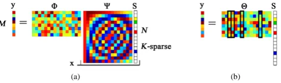
y= Φ +x υ (1) where, in the context of data compression, x∈RN is the N×1 vector representing the ECG signal, Φ ∈RM N×

(

M<N

)

is a user designed sensing matrix or measurement matrix, υ ∈RM is sensor noise, and y∈RM is the compressed signal. The matrix Φ here plays as a sensor that acquire information from the input signal x. The compressed signal, y, is sent to the receiver side where the original signal x is recovered by a CS algo-rithm using yand Φ. To successfully recover the ECG signal, x is required to be sparse. When x is not sparse, one generally seeks a sparsifying matrix or sparsifying dictionary Ψ such that x can be sparsely represented with the dictionary matrix, i.e., x= Ψz, where the representation coefficients z are sparse. Gener-ally, Ψ is constructed using some bases. In this paper, DWT basis is considered. Then a CS algorithm can first recover z using the available y and the M×N matrix Θ = ΦΨ. Then x can be recoverd according to x= Ψz. The basic CS framework has been widely used for ECG signals [6] [15]. Thus, equation (1) can be re-written in terms of the sparse signal coefficients as

(4)

x. The problem consists of designing a) a stable measurement matrix Φ such that the salient information in any K-sparse or compressible signal is not damaged by the dimensionality reduction from x∈RN to y∈RM and b) a reconstruction algorithm to recover 𝑥𝑥from only M ≈K measurements y (or about as many mea-surements as the number of coefficients recorded by a traditional transform coder). The key properties of the acquisition system in (2) are:

a) Instead of point evaluations of the signal, the system takes Minner products of the signal with the basis vector Φ;

b) The number of measurements M is considerably smaller than the number of signal coefficients N. If M =N , x can be recovered from z in a straightforward manner by inverting Θ. However, a recon-struction process is needed when M <N. In this case, the system is underdetermined, and there are an infinite number of feasible solutions for z. However, if the signal to be recovered is known to be sparse, then the sparsest solution (most 0’s) out of the infinitely possible is often the correct solution. The central result of the CS is that when the signal z has a sparse representation, and the measurements Φ are incoherent, the signal x can be reconstructed from y with a very high accuracy even when MN (M in the order of logN). The measurement matrix Φ can be chosen as noise-like, random matrix, which generally exhibits low-coherence with any representation basis. The savings in the number of measurements in practice are generally around

1 5 to

1

4 in typical acquisition systems, but much higher savings are achieved when the signals of interest have a highly sparse representation [3] [4].

After the acquisition process, an estimate of the signal is obtained by a reconstruction algorithm. A common and practical approach used to determine the sparse solution is to solve this problem as a convex optimization problem. The original work on CS employed regularization based on l₁-norms and linear programming, such that the signal is reconstructed using the following optimization problem [3] [4]:

1

minimize x subject to y= ΦΨz (3)

where

1

⋅ denotes the l₁-norm of a vector reinforcing a sparse solution, Ψ is the N×M basis matrix and

zis the coefficient vector. From (3), the recovered signal is then y= Ψx∗ where x∗ is the optimal solution. The l₁-norm cost function serves as a proxy for sparseness as it heavily penalizes small coefficients so the op-timization drives them to zero. The problem of minimizing the l₁-norm in (3) has been shown to be solved effi-ciently and requires only a small set of measurements

(

M N

)

to enable perfect recovery [16]. The implica-tion of these results is that an N-dimensional signal can be recovered from a lower order number of samples, M, provided that the signal is sparse in some basis. We rely on this result from CS theory to reduce the data that the sensor must transmit. Many other reconstruction algorithms have been proposed in the literature [17]-[19].

3. Measurement Matrices

The measurement matrix Φ must allow the reconstruction of the length-N signal x from M <N measure-ments (the vector y). Since M <N , this problem appears ill-conditioned. If, however, x is K-sparse and the K locations of the nonzero coefficients in z are known, then the problem can be solved provided M ≥K. A ne-cessary and sufficient condition for this simplified problem to be well conditioned is that, for any vector v shar-ing the same K nonzero entries as z and for some δ >s 0

(

)

2

(

)

2 2

2

1 _s v 1 _s

v

δ Θ δ

− ≤  ≤ +



(4)

(5)

mea-surements nearly linear in the sparsity level. Notice that the sensing matrix Φ does not depend on the signal. To guarantee robust and efficient recovery of the K-sparse signal, the sensing matrix Φ must obey the key re-stricted isometry property given by Equation (4).

A related condition, referred to as incoherence, requires that the rows of Φ cannot sparsely represent the columns of Ψ (and vice versa). The concept of coherence was introduced in a slightly less general framework by Donoho [3], and has since been used extensively in the field of sparse representations of signals. In particular, it is used as a measure of the ability of suboptimal algorithms such as matching pursuit and basis pursuit to cor-rectly identify the true representation of a sparse signal. Current assumptions in the field of compressed sensing and sparse signal recovery impose that the measurement matrix has uncorrelated columns. To be formal, the co-herence or the mutual coco-herence of a matrix A is defined as the maximum absolute value of the cross-correla- tions between the columns of A. Formally, let a a₁, ₂,,aN be the columns of the matrix A, which are

as-sumed to be normalized such that a aiT i =1. The mutual coherence of A is then defined as

( )

T

1maxi j m i j

A a a

µ

≤ ≠ ≤

= (5)

with a lower bound given by

( )

₍

₎

1

N d

A

d N

µ ≥ −

− (6)

We say that a dictionary is incoherent if

µ

( )

A is small. Standard results then require that the measurement matrix satisfy a strict incoherence property, as even the RIP imposes this. If the dictionary D is highly coherent, then the matrix AD will also be coherent in general.

Direct construction of a measurement matrix Φ such that Θ = ΦΨ has the RIP requires verifying (4) for each of the N

K    

  possible combinations of K nonzero entries in the vector v of length N. However, both the RIP and incoherence can be achieved with high probability simply by selecting Φ as a random matrix. For in-stance, let the matrix elements ϕ_{j i}_, be independent and identically distributed (iid) random variables from a Gaussian probability density function with mean zero and variance 1 N [3] [4]. Then the measurements y are merely M different randomly weighted linear combinations of the elements of x, as illustrated in Figure 1. The Gaussian measurement matrix Φ has two interesting and useful properties:

 The matrix Φ is incoherent with the basis Ψ =I of delta spikes with high probability. More specifically, an M×N iid Gaussian matrix Θ = ΦI can be shown to have the RIP with high probability if

(

)

log

M ≥cK N K , with c a small constant [3] [4]. Therefore, K sparse and compressible signals of length N can be recovered from only M ≥cKlog

(

N K

)

N random Gaussian measurements.

 The matrix Φis universal in the sense that Θ = ΦΨ will be iid Gaussian and thus has the RIP with high probability regardless of the choice of the orthonormal basis Ψ.

4. Signal Recovery from Incomplete Measurements

CS theory also proposes that rather than acquire the entire signal and then compress, it should be possible to capture only the useful information to begin with. The challenge then is how to recover the signal from what

[image:5.595.163.439.588.670.2]

(a) (b)

(6)

would traditionally seem to be an incomplete set of measurements. The ECG signal ˆx has to be recovered from the measurement vector y, with y being defined as in Equation (2). This poses a classical linear alge-bra problem. When does a unique solution exist to the set of linear equations y= Φx? Generally, a solution might exist for M ≤N, i.e., for a determined or over-determined system. Our case is one of a heavily under- determined system of equations and there are infinite solutions as a consequence. However, with additional known structure present in ECG signal, recovery can be attempted. In this case, with knowledge of signal spar-sity, a good approximation ˆx can be found, provided there are enough measurements. Again, the sparseness of the signal is relied upon to make this possible. So far, we have seen that if the signal of interest x is sparse, then it is possible to recover it from a number of measurements M <N . In this case, the system y= Φx is underdetermined and there are an infinite number of feasible solutions for x. However, if the signal to be re-covered is known to be sparse, then the sparsest solution (most 0’s) out of the infinitely possible is often the correct solution. A common and practical approach used to determine the sparse solution is to solve the convex optimization problem:

The question is now how we can actually recover x (or an estimate of it) from y, the problem being ill- posed. A common method, which is used for over determined systems of linear equations, is the Least Square (LS) approach, which is based on minimizing the residual energy. To enforce the a priori knowledge about sig-nal sparsity in the recovery algorithm, one should search for a solution with minimum l₀-norm. Since the l₀- norm counts the number of non-zero elements in a vector, minimizing it is equivalent to looking for the sparsest optimal solution x∗ which is in agreement with the measurements y. Unfortunately, this problem not only does not have a closed form solution, but it is also NP-hard to solve (combinatorial complexity). However, if we replace l₀-norm with l₁-norm, then the problem is convex and can be solved using standard convex optimiza-tion routines [20]. For this purpose, in this paper the solution to Equation (3) is found using l₁-magic software developed in [21].

It has been proven that computing the sparsest solution directly generally requires prohibitive computations of exponential complexity [22], so several heuristic methods have been developed in literature, such as Matching Pursuit (MP) [23], Basis Pursuit (BP) [24], log barrier method [20], iterative thresholding method [25], and so forth. Most of these methods or algorithms fall into three distinct categories: greedy algorithms, l₁-minimization, and TV minimization.

4.1. Greedy Algorithms

Generally speaking, a greedy algorithm refers to any algorithm following the metaheuristic of choosing the best immediate or local optimum at each stage and expecting to find the global optimum at the end. It can find the global optimum for some optimization problems, but not for all [20]. This algorithm decomposes any signal into a linear combination of waveforms in a redundant dictionary of functions so that selected waveforms optimally match the structure of the signal. MP is easy to implement and has an exponential rate of convergence and good approximation properties. However, there is no theoretical guarantee that MP can achieve sparse representations. In [26], the authors proposed a variant of MP, Orthogonal Matching Pursuit (OMP), which guarantees the nearly sparse solution under some conditions. A primary drawback of MP and its variants is the incapability of attain-ing truly sparse representations. The failure is usually caused by an inappropriate initial guess. This shortcomattain-ing also motivated the development of algorithms based on l₁-minimization.

4.2. l

1

-Minimization Algorithms

In [3] some early results related to l₁-minimization for signal recovery have been introduced. The question why

1

l -minimization could work in some special setups was further investigated and answered in [20] [21]. Specifi-cally, a signal which is K-sparse under some basis can be exactly recovered from c K linear measurements by l₁- minimization under some conditions, where c is a constant. The new CS theory has significantly improved those earlier results. How big the constant c is here directly decides the size of linear measurements, important infor-mation needed to encode or decode a signal. The introduction of the concept RIP for matrices [4] [5] showed that if the measurements satisfy the RIP of a certain degree, it is sufficient to recover the sparse signal exactly from its decoded signal. However, it is extremely difficult to verify the RIP property in practice. Fortunately, Cand’es et al. in [15] showed that RIP holds with high probability when the measurements are random. Usually

1

(7)

seeks the solution that minimizes the l₁-norm of the coefficients, is a prototype of l₁-minimization. BP can simply be comprehended as linear programming solved by some standard methods. Furthermore, BP can com-pute sparse solutions in situations where greedy algorithms fail. All this work enriches the significance of stud-ying and applstud-ying l₁-minimization and compressive sensing in practice.

The solution to the above problem can be found with relative ease. There are methods that will find the solu-tion to the BP problem but does it lead to a sparse solusolu-tion? The answer in general is no but under the right con-ditions it can be guaranteed that BP will find a sparse solution or even the sparsest solution. This is because l₁- norm is only concerned with the value of entries not the quantity. A vector with a small l₁ could have very small valued non zero entries in every position which would give it a large l₀-norm. There are numerous algo-rithms to solve the problems involving the l₁-norm. One of these algorithms that has been used to solve this convex optimization problem is implemented in the Matlab software package CVX, a package for solving con-vex problems [27]. Simplex and interior-point methods offer an interesting insight into these optimization prob-lems and will be introduced in the following. The standard simplex method starts by forming a new matrix A∗ consisting of linearly independent columns of A. Since all the columns of A∗ are independent b can be uni-quely represented (or approximated) with respect to A∗. Then an iteration process takes place, where at each iteration a column vector of A∗ is swapped with a column vector of A. Each swap improves the desired prop-erty of the solution. In this case a reduction of the value of the l₁-norm. The interior method starts with a solu-tion x₀ where Ax₀ =b. Then goes through an iteration process changing the entries in x_k−₁ to form a new solution x_k while maintaining the condition Ax_k =b. A transformation is then applied to x_k which effec-tively sparsifies x_k. Eventually a vector is reached that meets the preset stopping conditions and by forcing all extreme small entries to zero, the final solution is obtained.

4.3. TV Minimization Algorithms

In the broad area of compressive sensing, l₁-minimization has attracted intensive research activities since the discovery of l l₀ ₁ equivalence [3]-[5]. However, for image restoration, recent research has confirmed that the use of Total Variation (TV) regularization instead of the l₁ term in CS problems makes the recovered image quality sharper by preserving the edges or boundaries more accurately, which is essential to characterize images. The advantages of TV minimization stem from the property that it can recover not only sparse signals or images, but also dense staircase signals or piecewise constant images. In other words, TV regularization would succeed when the gradient of the underlying signal or image is sparse. Even though this result has only been theoretically proven under some special circumstances [4], it stands true on a much larger scale empirically. A detailed dis-cussion on TV models has been reported by Chambolle et al. [28]. However, the properties of non-differentia- bility and non-linearity of TV functions make them far less accessible computationally than solving l₁-minimization models. In 2004, Chambolle [29] proposed an iterative algorithm for TV denoising and proved the li-near convergence. Furthermore, Chambolle’s algorithm can be extended to solve image reconstruction problems with TV regularization while the measurement matrix is orthogonal. Due to the powerful application of TV re-gularization in the edge-detection and many other fields, researchers kept trying for several years to explore al-gorithms for solving TV minimization problems. However, these alal-gorithms are still either much slower or less robust compared with algorithms designed for l₁-minimization.

5. Sparse Representation of ECG Signal

(8)

This section introduces the wavelet transformation technique used for controlling the ECG signal sparisty. The wavelet transform describes a multi-resolution decomposition process in terms of expansion of a signal onto a set of wavelet basis functions. Wavelet transforms have become an attractive and efficient tool in many applications especially in coding and compression of signals because of multi-resolution and high-energy com-paction properties. Wavelets allow both time and frequency analysis of signals simultaneously because of the fact that energy of wavelet is concentrated in time and still possesses the wave like characteristics. As a result wavelet representation provides a versatile mathematical tool to analyze ECG signals.

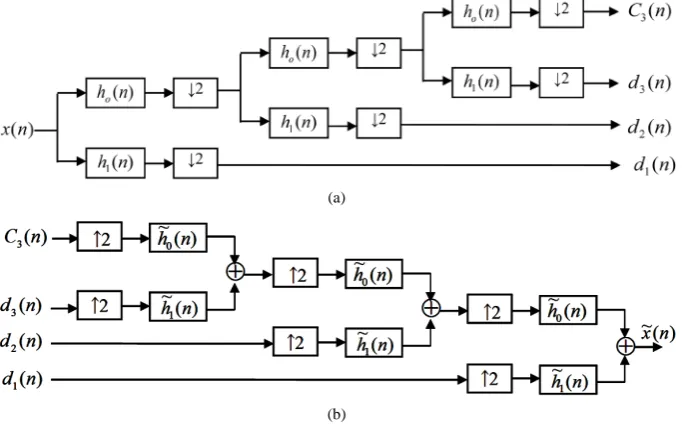
Discrete Wavelet Transformation (DWT) has its own excellent space frequency localization property. The key issues in DWT and inverse DWT are signal decomposition and reconstruction, respectively. The basic idea behind decomposition and reconstruction is low-pass and high-pass filtering with the use of down sampling and up sampling respectively. The result of wavelet decomposition is hierarchically organized decompositions. One can choose the level of decomposition j based on a desired cutoff frequency. Figure 2(a)shows an imple-mentation of a three-level forward DWT based on a two-channel recursive filter bank, where h n0

( )

and

( )

1

h n are low-pass and high-pass analysis filters, respectively, and the block 2 represents the down sampling operator by a factor of 2. The input signal x n

( )

is recursively decomposed into a total of four subband signals: a coarse signal C n3

( )

, and three detail signals, D n3

( )

, D n2

( )

, and D n1

( )

, of three resolutions. Figure 2(b)

shows an implementation of a three-level inverse DWT based on a two-channel recursive filter bank, where

( )

0

h n and h n1

( )

are low-pass and high-pass synthesis filters, respectively, and the block 2 represents the up

sampling operator by a factor of 2. The four subband signals C n3

( )

, D n3

( )

, D n2

( )

and D n1

( )

, are recur-

sively combined to reconstruct the output signal x n

( )

. The four finite impulse response filters satisfy the following relationships:

( ) ( ) ( )

1 1 0

n

h n = − h n (7)

( )

(

)

0 0 1

h n =h −n (8)

( ) ( ) (

)

1 1 0 1

n

h n = − h −n (9) so that the output of the inverse DWT is identical to the input of the forward DWT. In this environment, ECG signal representation using a wide variety of wavelets, drawn from various families including symlets and Dau-bechies’ bases has been adopted. In this context, the transform coefficients are arranged in decreasing order of magnitude, and count the number of coefficients accounting for 99% of the signal energy (as parser representa-tion requires less number). “Symlet” and “Daubechies” families generally offer more compact representarepresenta-tion compared to Meyer wavelet as well as biorthogonal and reverse biorthogonal families. In particular, the sparsest re-

(a)

[image:8.595.129.471.493.705.2]

(b)

(9)

presentation is provided by the “sym4” (closely followed by the “db4”) wavelet basis for abroad class of ECG signals [30]-[32].

6. Improving ECG Signal Sparisty Using QRS-Complex Estimation

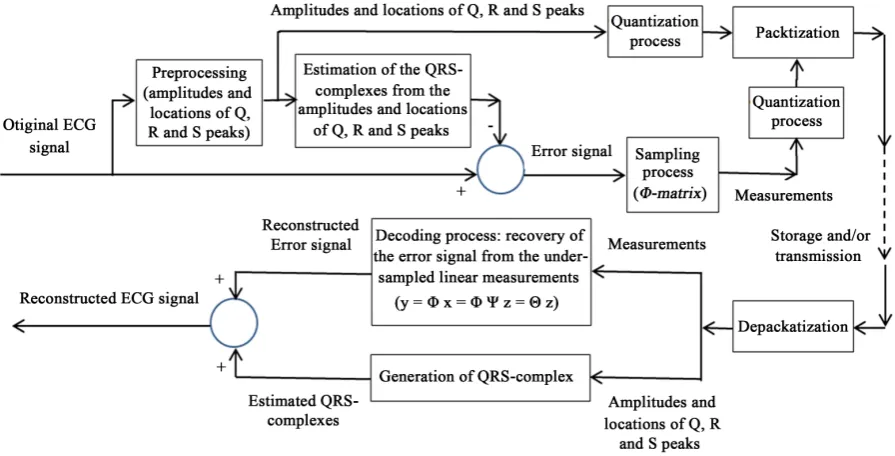
The correlation between the consecutive ECG beats can be exploited to improve the ECG signal sparisty. For this purpose, in this paper, the QRS-complex has been estimated based on the peaks and locations of Q, R and S waves. Then the estimated QRS-complex is subtracted from the original ECG signal and the resulting differential signal is manipulated using CS technique. The proposed compression scheme is presented inFigure 3. The details of the purposed compression algorithm are illustrated in subsequent steps as follows.

1) The signal is decomposed into windows; each of length 1024 samples. This short window length is considered in order to generate an approximate real time transmission. At the same time, many heartbeats in the window are incorporated to recover the signal with fewer samples.

2) The signal is preprocessed to determine the amplitudes and locations of the Q, R and S peaks. These para-meters are used to estimate the QRS-complexes.

3) From the estimated QRS-complexes and the locations of the R-peaks locations, the error signal with more sparisity compared to the original ECG signal is determined as the difference between the original ECG signal and the estimated QRS-complexes.

4) Fewer measurements are determined from the resulting error signal and the sensing matrix. 5) The amplitudes and locations of the Q, R and S peaks and the measurement matrix are quantized. 6) The resulting quantized values are packetized for possible storage and/or transmission.

6.1. Preprocessing

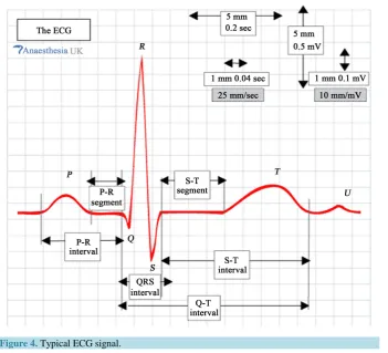
[image:9.595.90.538.477.705.2]

In this section, the signal sparisty is controlled through the extraction of the significant ECG signal features. These features are extracted by estimating the QRS-complex for each signal beat. Then, the estimated QRS-complex is subtracted from the original ECG signal. After that, the resulting error signal is transformed into DWT domain and the resulting transformed coefficients are compressed using CS technique. A typical scalar ECG heartbeat is shown in Figure 4. The significant features of the ECG waveform are the P, Q, R, S and T waves and the dura-tion of each wave. A typical ECG tracing of electrocardiogram baseline voltage is known as the isoelectric line. It is measured as the portion of the tracing following the T wave and preceding the next P wave. In addition to the QRS-complex, the ECG waveform contains P and T waves, 50-Hz noise from power line interference, EMG signal from muscles, motion artifact from the electrode and skin interface, and possibly other interference from

(10)

[image:10.595.127.479.82.401.2]

Figure 4. Typical ECG signal.

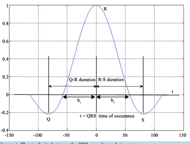
electro surgery equipment. The power spectrum of the ECG signal can provide useful information about the QRS-complex estimation. Figure 5summarizes the relative power spectra, based on the FFT, of the ECG, QRS- complex, P and T waves, motion artifact, and muscle noise taken for a set of 512 sample points that contain ap-proximately two heartbeats [33]. It is visible that QRS-complex power spectrum involves the major part of the ECG heartbeat. Normal QRS-complex is 0.06 to 0.1 sec in duration and not every QRS-complex contains a Q wave, R wave, and S wave. By convention, any combination of these waves can be referred to as a QRS-complex. This portion can be represented by Q, R and S values, the Q-R and R-S durations and the event time of R as shown in Figure 4. These values can be extracted from the original signal.

6.2. The QRS-Complex Detection and Estimation

The aim of the QRS-complex estimation is to produce typical QRS-complex waveform using parameters ex-tracted from the original ECG signal [34]. The estimation algorithm is a Matlab based estimator and is able to produce normal QRS waveform. A single heartbeat of ECG signal is a mixture of triangular and sinusoidal waveforms. The QRS-complex waveform can be represented by shifted and scaled versions of these waveforms.

Figure 6illustrates a sinc function that looks like the QRS-complex. However, in QRS-complex the QR-duration is not equal to the RS-duration. So, the QRS estimation is divided into two parts: QR part and RS part. The QR part can be generated using a sinc function described by

( )

1 1

1

sin t , 0 F x A c

b b t

 

= _ _ − <

 <

 (10) where, b₁ is the QR duration and A₁ is a scaling factor determined as the difference between the R-peak and the Q-peak. Similarly, the RS part is generated using a sinc function described by

( )

2 2

2

sin t , 0

F x A c

b t b

 

= _ _ < <

(11)

[image:11.595.160.440.85.280.2] [image:11.595.137.462.314.560.2]

Figure 5. Relative power spectra of QRS-complex, P and T waves, and mus-cle noise and motion artifacts [33].

Figure 6. The similarity between the QRS-complex and sinc wave.

where, b₂ is the RS duration and A₂ is a scaling factor determined as the difference between the R-peak and the S-peak. The two parts are combined beside each other to form the estimated QRS signal. Finally, using the R occurrence time the estimated signal is time shifted to fit the occurrence time of the original signal.

(12)

(a)

(b)

[image:12.595.128.466.80.390.2]

(c)

Figure 7. The first 1000 sample of record 100. (a) The original signal; (b) The estimated QRS- complex; (c) Difference between the original and the estimated QRS-complex signal.

Table 1. The values of peaks of the Q, R and S waves as well as the RR-periods’ durations.

Values and durations

Period number

1 2 3 4

Q-values −0.0469 −0.0537 −0.0483 −0.0464

R-values 0.3027 0.3013 0.2808 0.2983

S-values −0.0376 −0.0415 −0.0449 0.0493

QR-duration 12 12 13 12

RS-duration 10 8 8 5

7. Performance Metrics & Quality Measurement

A practical compression algorithm should not focus totally on compression itself. Many applications have re-quirements for the quality of the de-compressed signal. A robust compression algorithm should have the ability to maintain the quality of the de-compressed signal while achieving reasonable compression ratio. This is be-cause only good quality signal reconstruction makes sense in reality. The evaluation of performance for testing ECG compression algorithms includes three components: compression efficiency, reconstruction error and computational complexity. All data compression algorithms minimizes data storage by reducing the redundancy wherever possible, thereby increasing the Compression Ratio (CR). Thus, the compression efficiency is meas-ured by the CR. The compression ratio and the reconstruction error are usually dependent on each other. The computational complexity component is part of the practical implementation consideration. The following eval-uation metrics were employed to determine the performance measures of the proposed method [1] [2]. The CR is defined as the ratio of the number of bits representing the original signal to the number of bits required to

0 200 400 600 800 1000 1200

0 0.2 0.4

The original ECG signal

A

m

pl

it

ude

0 200 400 600 800 1000 1200

0 0.2 0.4

The estimated QRS -complex

A

m

pl

it

ude

0 200 400 600 800 1000 1200

0 0.2 0.4

The difference between the ECG signal and the estimated QRS -complex

S ample Index

A

m

pl

it

[image:12.595.90.544.443.558.2]

(13)

store the compressed signal.

orig

comp

CR% b 100

b

= ∗ (12)

where b_orig and b_comp represent the numbers of bits required for the original and compressed signals, respec-tively. A high compression ratio is typically desired. A data compression algorithm must also represent the data with acceptable fidelity while achieving high CR.

Quality of lossy compression schemes is usually determined by comparing the de-compressed data and the original data. If there are no differences at all, then the compression is lossless. Conventional measurements are based on mathematical distortions, such as percentage root mean square difference (PRD) and signal-to-noise ratio (SNR), etc. These measurements are not specific for ECG signals; they reflect the distortion of signal by statistics criteria. They are of general purpose, so the criteria may not be very accurate to describe the characte-ristics of a specific signal type.

For example, the ECG signal is for medical use, so what concerns medical specification most is the diagnostic feature, which is not covered in the general mathematical descriptions. Thus, in [37] the Weighted Diagnostic Distortion (WDD) is proposed. It uses diagnostic features as criteria and has better feedback from the perspec-tive of medical specialists than other measurements. However, WDD may not bring the benefit and it is far more complex. Table 2 shows a comparison between different quality measures. Among those, PRD is the most widely used measure in ECG data compression. PRD, SNR and STD are mathematically related. PRD is derived from RMSE, which measures the power of errors between the original data and the reconstructed data and is used frequently for prediction. The advantage of the PRD over RMS is its scale-independence. That makes PRD more accurate across different data sets. The PRD indicates the error between the original ECG samples and the reconstructed data. This metric is commonly used for measuring the distortions in reconstructed biomedical signals such as ECG signals and EEG signals. There are subtle differences in calculation; PRD has 3 types for ECG data compression, which are numbered 0, 1, and 2. The definitions are described by Equations (13), (14) and (15) for signal x of length N samples.

( )

(

)

( )

(

)

2 orig recon 1 0 2 orig 1

PRD % 100

N i

x i x i

x i

=

= −

=

∑

×

∑

(13)

( )

(

)

( )

(

)

PRD % 100

offset

N i

x i x i

x i = = − = × −

∑

(14)

( )

(

)

( )

(

)

PRD % 100

N i

x i x i

x i x

= = − = × −

∑

[image:13.595.94.316.565.722.2]

∑

(15)

Table 2. Comparison between different quality measures.

Measurement Definition Feature

PRD Percentage root mean square difference

RMSE Root mean square error

SNR Signal to noise ratio Often used for data transmission

STD Standard deviation

QS Quality score

CC Cross correlation Evaluate the similarity between the original signal and its reconstruction

MAXERR Maximum error

PARE Peak amplitude related error

(14)

where, xorig

( )

i is the sampled values of the original signal, xrecon

( )

i is the sampled values of the

recon-structed/predicted signal and x is the mean value of x. Compare to PRD₀, PRD₁ is optimized by sub-tracting the offset, which is usually added from database for data storage. For the MIT-BIH database the offset is 1024. PRD₂ is further optimized by subtracting the mean value (approximately the DC component). The result is thus more accurate removing a lot of effects from DC offset. It should be noticed that PRD₁ is more popular in literature because of its simplicity but PRD₂is preferred because it is more accurate. Table 3shows the con-nection between the quality indication and the PRD values

(

PRD1

)

[37].

The CR and PRD have the close relationship in the lossy compression algorithms. In general, the CR goes higher with the higher lossy level, while the error rate goes up. The final goal of the proposed compression algo-rithm is to keep the PRD value smaller than that of the conventional methods while maintaining the similar CR. Thus, quality score defined as the ratio between CR and PRD (QS = CR/PRD) is sometimes used to quantify the overall performance of the compression algorithm, considering both the CR and the error rate. A high score represents a good compression performance. Another distortion metric is the root mean square error (RMSE). In data compression, we are interested in finding an optimal approximation for minimizing this metric as defined by the following formula:

( )

(

)

2

orig recon 1

RMSE 100

N

i x i x i

N

= −

=

∑

× (16)

Since the similarity between the reconstructed and original signal is crucial from the clinical point of view, the cross correlation (CC) is used to evaluate the similarity between the original signal and its reconstruction.

( )

(

)

(

( )

)

( )

(

)

(

( )

)

orig orig recon recon 1

2 2

orig orig recon recon 1

1

CC 1

N i N i

x i x i x i x i

N

x i x i x i x i

N =

=

  ₋ ₋

    =

  ₋ ₋

   

∑

(17)

where x_orig

( )

i and x_recon

( )

i are the mean values of the original and reconstructed signals, respectively. In order to understand the local distortions between the original and the reconstructed signals, two metrics, the max-imum error (MAXERR) and the peak amplitude related error (PARE), should be computed. The maxmax-imum error metric is defined as

( )

(

orig recon

)

MAXERR=max x i −x i , i=1, 2,,N (18) and it shows how large the error is between every sample of the original and reconstructed signals. This metric should ideally be small if both signals are similar. The PARE is defined as

( )

(

orig

( )

recon

( )

)

orig

( )

PARE i = x i −x i x i , i=1, 2,,N (19) By plotting PARE, one will be able to understand the locations and magnitudes of the errors between the original and reconstructed signals.

8. Experimental Results

[image:14.595.128.471.620.720.2]

Compressive sensing directly acquires a compressed signal representation without going through the interme-diate stage of acquiring N samples, where N is the signal length. Since CS-based techniques are still in early

Table 3. PRD ranges and quality connection. ₁

Range of PRD % 1 Quality

1 PRD

0%≤ %<2% Very good

1 PRD

2%≤ %<9% Good

1

9%≤PRD%<19% Not good

1 PRD

(15)

stages of research and development, specially the development of Analog to Information Conversion (AIC) hardware, signals that are used for experimentation are acquired in the traditional way. The CS measurements of these data are computed from the original ECG signal. Tests were conducted using 10-min long single-lead ECG signal extracted from records 100, 107, 115 and 117 in the MIT-BIH Arrhythmia database. Record 115 is in-cluded in the data set to evaluate the performance of the algorithm in the case of irregular heartbeats. The data are sampled with 360 Hz and each sample is represented with 11-bit resolution. The records are split into non- overlapping 1024 samples windows that are processed successively. Then the characteristic points of the ECG waveforms are detected using the procedure introduced in Section 6.2. It relies on the extraction of Q, R and S peaks and locations and the estimation of the QRS-complex. We begin by first detecting the R peaks, since they yield modulus maxima with highest amplitudes. This enables the segmentation of the original ECG record into individual beats. Then, multi scale wavelet decomposition is performed on the difference between the given ECG window, and the estimated QRS-complexes.

To evaluate the performance of the proposed method concerning the amount of data compression, the sparisi-ty of the ECG signal in both the time-domain and the wavelet-domain are measured. As it has been mentioned before, the sparisity of an array x is defined as the number of non-zero entries in x. For this purpose two ECG signals, each of length 6 seconds, extracted from records 100 and 106 of the MIT-BIH database are considered.

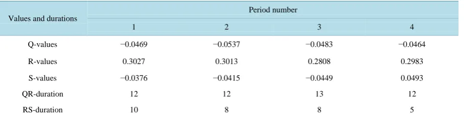
[image:15.595.89.530.465.682.2]

Figure 8 illustrates the time-domain representation of the two ECG signals, their estimated QRS-complexes and the differences between them. Figure 9illustrates the threshold wavelet coefficients of the original ECG signal, and that of the differences between the original signal and the estimated QRS-complex for the two records. The bi-orthogonal wavelet filter “bior4.4” has been adopted in the wavelet transformation process where the de-composition has been carried out up to the 8th level. Thresholding is performed such that 98% of the total coeffi-cients’ energy is kept and small coefficients are thrown away.

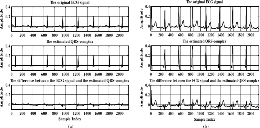
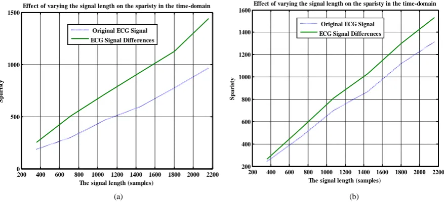
Figure 10illustrates the effect of varying the signal length on the sparisity of the time-domain representation of ECG signals and the signals differences of the records after thresholding each of them such that 98% of the total energy is kept and small samples are thrown away. From this Figure it can be concluded that increasing the signal length increases its sparisity. Moreover, the signals differences are sparser compared to the original sig-nals. Figure 11shows the effect of varying the signal length on the sparisity of the wavelet representation of the ECG signals and the signals differences of the two records after thresholding both of them. Comparing the re-sults presented in Figure 10and Figure 11shows that the wavelet transformed signals are sparser compared to the signal in time-domain.

(a) (b)

Figure 8. Time-domain representation of the original ECG signal, the estimated QRS-complex and the differences be-tween the original signal, the estimated QRS-complex for two MIT-BIH records. (a) For MIT-BIH record 100; (b) For MIT-BIH record 106.

0 200 400 600 800 1000 1200 1400 1600 1800 2000 0

0.2 0.4

A

m

pl

it

ude

0 200 400 600 800 1000 1200 1400 1600 1800 2000 0

0.2 0.4

The estimated QRS-complex

A

m

pl

it

ude

0 200 400 600 800 1000 1200 1400 1600 1800 2000 0

0.2 0.4

The difference between the ECG signal and the estimated QRS-complex

Sample Index A m pl it ude

0 200 400 600 800 1000 1200 1400 1600 1800 2000 0

0.2 0.4

A

m

pl

it

ude

0 200 400 600 800 1000 1200 1400 1600 1800 2000 0

0.2 0.4

The estimated QRS-complex

A

m

pl

it

ude

0 200 400 600 800 1000 1200 1400 1600 1800 2000 0

0.2 0.4

The difference between the ECG signal and the estimated QRS-complex

(16)

[image:16.595.82.534.81.298.2]

(a) (b)

Figure 9. Wavelet representation of both the original ECG signal, and the differences between the original signal, the esti-mated QRS-complex for two MIT-BIH records. (a) For MIT-BIH record 100; (c) For MIT-BIH record 106.

[image:16.595.92.531.338.538.2]

(a) (b)

Figure 10. Effect of varying the signal length on the sparisity of the time-domain representation of ECG signals extracted from two MIT-BIH records. (a) For MIT-BIH record 100; (c) For MIT-BIH record 106.

Figure 12 illustrates the effect of varying the number of decomposition levels on the sparisity of the wavelet- domain representation of the original ECG signals and the signal differences of two MIT-BIH records. It shows that for record 100, the original signal is sparser than the signal differences for decomposition levels below 7. Otherwise, the signal differences are sparser. However, for record 106, the original signal is sparser than the signal differences for decomposition levels below 5. Otherwise, the signal differences are sparser. This indicates that the sparisity of the signal differences depends on the number of decomposition levels.

Figure 13illustrates the effect of selecting the wavelet filters on the sparisity of the wavelet-domain repre-sentation of the original ECG signals and the signal differences extracted from two MIT-BIH records. It shows that for both records, the signal differences are sparser compared to the original signal for all Daubechies’ filters (from db2 up to db10). Comparing the results presented in Figure 13(a)and Figure 13(b)shows that the sparis-ity of the wavelet transformed signals depends on the ECG record to be analyzed. This has been checked by considering other MIT-BIH records.

0 500 1000 1500 2000

-0.1 0 0.1 0.2 0.3

The thresholded wavelet coefficients of the original ECG signal

A

m

pl

it

ude

0 500 1000 1500 2000

-0.1 0 0.1 0.2 0.3

The thresholded wavelet coefficients of the differences signal

A

m

pl

it

ude

0 500 1000 1500 2000

-0.1 0 0.1 0.2 0.3

The thresholded wavelet coefficients of the original ECG signal

A

m

pl

it

ude

0 500 1000 1500 2000

-0.1 0 0.1 0.2 0.3

The thresholded wavelet coefficients of the differences signal

A

m

pl

it

ude

200 400 600 800 1000 1200 1400 1600 1800 2000 2200 0

500 1000 1500

Effect of varying the signal length on the sparisty in the time-domain

The signal length (samples)

Spa

ri

st

y

Original ECG Signal ECG Signal Differences

200 400 600 800 1000 1200 1400 1600 1800 2000 2200 200 400 600 800 1000 1200 1400 1600

Effect of varying the signal length on the sparisty in the time-domain

Spa

r

is

ty

(17)

[image:17.595.77.534.82.300.2]

(a) (b)

Figure 11. Effect of varying the signal length on the sparisity of the wavelet-domain representation of ECG signals ex-tracted from two MIT-BIH records. (a) For MIT-BIH record 100; (c) For MIT-BIH record 106.

(a) (b)

Figure 12. Effect of varying the number of decomposition levels on the sparisity of the wavelet-domain representation of the original ECG signals and the signal differences extracted from two MIT-BIH records. (a) For MIT-BIH record 100; (b) For MIT-BIH record 106.

To explore the effect of controlling the signal sparisity using other wavelet families, sparse representation is checked using bi-orthogonal (bior4.4) DWT filters and compared with that using Daubechies (db6) filters. In both cases the transformation is performed with four detailed levels and one approximation level. Another im-portant process is also considered to improve the signal sparasity; that is by thresholding the wavelet coefficients in different decomposition levels according to the energy content in each subband. In this case, the wavelet coefficients have been thresholded to preserve 98%, 96%, 94% and 90% of the coefficients energy in the 1st, 2nd, 3rd, and 4th details subbands respectively. Moreover, the coefficients in the approximation subband are kept without threshold. After that, the resulting wavelet coefficients are mapped into significant and insignificant coefficients by ones and zeros respectively.

Figure 14illustrates wavelet coefficients before and after thresholding of the transformed difference between 200 400 600 800 1000 1200 1400 1600 1800 2000 2200

10 20 30 40 50 60 70 80 90 100

Effect of varying the signal length on the sparisty in the wavelet-domain

Spa

r

is

ty

DWT Coefficients of Original ECG Signal DWT Coefficients of ECG Signal Differences

200 400 600 800 1000 1200 1400 1600 1800 2000 2200 20

30 40 50 60 70 80 90 100

Effect of varying the signal length on the sparisty in the wavelet-domain

Spa

r

is

ty

2 3 4 5 6 7 8 9 10

0 50 100 150 200 250 300

Effect of varying the number of decomposition levels on the wavelet sparisty

The number of decomposition levels

Spa

r

is

ty

2 3 4 5 6 7 8 9 10

0 50 100 150 200 250

Effect of varying the number of decomposition levels on the wavelet sparisty

The number of decomposition levels

Spa

r

is

ty

[image:17.595.89.531.338.553.2]

(18)

[image:18.595.87.505.84.289.2]

(a) (b)

Figure 13. Effect of varying the Daubechies’ filters on the wavelet sparisty of the wavelet-domain representation of the original ECG signals and the signal differences extracted from two MIT-BIH records. (a) For MIT-BIH record 100; (b) For MIT-BIH record 106.

(a) (b)

Figure 14. The wavelet coefficients before and after thresholding of the transformed difference between the original and the estimated QRS-complex together with the mapping of the significant coefficients. (a) For Daubechies db6 wavelet filter; (b) For Biorthogonal bior4.4 wavelet filter.

the original ECG signal and the estimated QRS-complex together with the mapping of the significant and insig-nificant coefficients for the two wavelet filters. The ECG signal considered here is of length 1200 samples ex-tracted from record 103.

Next, the performance of the proposed compression method has been compared with traditional wavelet based ECG compression techniques. Table 4 illustrates the comparison between the performances of the proposed method and two other methods for the compression of four MIT-BIH ECG records (100, 107, 115 and 117) [15] [36]. The proposed method is tested for the compression of the original signal and the signal differences using the CS technique and bior4.4 wavelet filters and eight decomposition levels. For all cases, the same signal length of 1024 samples is used. As illustrated in the table, the proposed method achieves better results in terms of the CR and PRD. Moreover, the results of the proposed indicate that the signal differences is compressed more than the original signal and smaller PRD₁. Figure 15 shows the performance of the proposed CS compressor

2 3 4 5 6 7 8 9 10

15 20 25 30 35 40 45 50 55

Effect of varying the Daubechies' filters on the wavelet sparisty

The order of the Daubechies filter

Spa

r

is

ty

2 3 4 5 6 7 8 9 10

30 35 40 45 50 55 60 65

Effect of varying the Daubechies' filters on the wavelet sparisty

The order of the Daubechies filter

Spa

r

is

ty

0 200 400 600 800 1000 1200

-0.2 0 0.2

The wavelet coefficients before Thresholding

A

m

pl

it

ude

0 200 400 600 800 1000 1200

-0.2 0 0.2

The wavelet coefficients after Thresholding

A

m

pl

it

ude

0 200 400 600 800 1000 1200

0 0.5 1 1.5

The mapping of the significant and insignificant wavelet coefficients

Coefficient Index A m pl it ude

0 200 400 600 800 1000 1200

-0.2 0 0.2

The wavelet coefficients before Thresholding

A

m

pl

it

ude

0 200 400 600 800 1000 1200

-0.2 0 0.2

The wavelet coefficients after Thresholding

A

m

pl

it

ude

0 200 400 600 800 1000 1200

0 0.5 1 1.5

The mapping of the significant and insignificant wavelet coefficients

[image:18.595.86.512.336.542.2]

(19)

[image:19.595.156.444.85.342.2]

Figure 15. The performance of the proposed CS based technique.

Table 4. Comparison of the proposed method using Compressed Sensing with two other compression methods for four MIT-BIH ECG records (100, 107, 115 and 117).

Record number Reference CR PRD1 %

Record 100

The proposed method (signal differences) 12.37 1.07

The proposed method (original ECG signal) 9.06 1.62

Polania et al., [15] 8.49 6.09

Lu et al., [36] 8.42 6.19

Record 107

Polania et al., [15] 8.19 6.05

Lu et al., [36] 8.13 6.12

Record 115

Polania et al., [15] 8.65 5.92

Lu et al., [36] 8.73 5.84

Record 117

Polania et al., [15] 7.23 2.57

Lu et al., [36] 7.23 2.57

in compressing 1024 samples of the signal differences. This figure indicates that the proposed method achieved low reconstruction error. This corresponds to high quality recovered ECG signal and even outperforms the two other techniques [15] [36].

0 200 400 600 800 1000 1200

1000 1200 1400

A

m

pl

it

ude

0 200 400 600 800 1000 1200

1000 1200 1400

The reconstructed ECG signal

A

m

pl

it

ude

0 200 400 600 800 1000 1200

-200 0 200

The difference between the original and reconstructed ECG signal

S ample Index

A

m

pl

it

[image:19.595.93.539.379.674.2]

(20)

9. Conclusion

This paper investigates CS approach as a revolutionary acquisition and processing theory that enables recon-struction of ECG signals from a set of non-adaptive measurements sampled at a much lower rate than required by the Nyquist-Shannon theorem. This results in both shorter acquisition times and reduced amounts of ECG data. At the core of the CS theory is the notion of signals sparseness. The information contained in ECG signals is represented more concisely in DWT transform domain and its performances in compressing ECG signals are evaluated. By acquiring a relatively small number of samples in the “sparse” domain, the ECG signal can be re-constructed with high accuracy through well-developed optimization procedures. Simulation results validate the superior performance of the proposed algorithm compared to other published algorithms. The performance of the proposed algorithm, in terms of the reconstructed signal quality and compression ratio, is evaluated by adopting DWT spatial domain basis applied to ECG records extracted from the MIT-BIH Arrhythmia Database. The results indicate that average compression ratio of 11:1 with PRD₁=1.2% are obtained. Moreover, the ad-vantage of the proposed method is that the quality of the retrieved signal is guaranteed and the compression ratio achieved is an improvement over those obtained by previously reported CS based algorithms. Simulation results suggest that CS should be considered as an acceptable methodology for ECG compression.

References

[1] Addison, P.S. (2005) Wavelet Transforms and the ECG: A Review. Physiological Measurement, 26, R155-R199. http://dx.doi.org/10.1088/0967-3334/26/5/R01

[2] Abo-Zahhad, M.M., Abdel-Hamid, T.K. and Mohamed, A.M. (2014) Compression of ECG Signals Based on DWT and Exploiting the Correlation between ECG Signal Samples. International Journal of Communications, Network and System Sciences, 7, 53-70. http://dx.doi.org/10.4236/ijcns.2014.71007

[3] Donoho, D.L. (2006) Compressed Sensing. IEEE Transactions on Information Theory, 52, 1289-1306. http://dx.doi.org/10.1109/TIT.2006.871582

[4] Candes, E., Romberg, J. and Tao, T. (2006) Robust Uncertainty Principles: Exact Signal Reconstruction from Highly Incomplete Frequency Information. IEEE Transactions on Information Theory, 52, 489-509.

http://dx.doi.org/10.1109/TIT.2005.862083

[5] Candes, E.J. and Wakin, M.B. (2008) An Introduction to Compressive Sampling. IEEE Signal Processing Magazine,

25, 21-30. http://dx.doi.org/10.1109/MSP.2007.914731

[6] Mamaghanian, H., Khaled, N., Atienza, D. and Vandergheynst, P. (2011) Compressed Sensing for Real-Time Ener-gy-Efficient ECG Compression on Wireless Body Sensor Nodes. IEEE Transactions on Biomedical Engineering, 58, 2456-2466. http://dx.doi.org/10.1109/TBME.2011.2156795

[7] Chen, F., Chandrakasan, A.P. and Stojanovic, V.M. (2012) Design and Analysis of a Hardware-Efficient Compressed Sensing Architecture for Data Compression in Wireless Sensors. IEEE Journal of Solid-State Circuits, 47, 744-756. http://dx.doi.org/10.1109/JSSC.2011.2179451

[8] Dixon, A.M.R., Allstot, E.G., Gangopadhyay, D. and Allstot, D.J. (2012) Compressed Sensing System Considerations for ECG and EMG Wireless Biosensors. IEEE Transactions on Biomedical Circuits and Systems, 6, 156-166.

http://dx.doi.org/10.1109/TBCAS.2012.2193668

[9] Polania, L.F., Carrillo, R.E., Blanco-Velasco, M. and Barner, K.E. (2012) Compressive Sensing Exploiting Wavelet Domain Dependencies for ECG Compression. Proceedings of the SPIE Defense, Security, and Sensing, Baltimore, 23-27 April 2012, 83650E.

[10] Polania, L.F., Carrillo, R.E., Blanco-Velasco, M. and Barner, K.E. (2012) On Exploiting Interbeat Correlation in Com-pressive Sensing-Based ECG Compression. Proceedings of the SPIE Defense, Security, and Sensing, Baltimore, 23-27 April 2012, 83650D

[11] Polania, L.F., Carrillo, R.E., Blanco-Velasco, M. and Barner, K.E. (2012) Compressive Sensing for ECG Signals in the Presence of Electromyography Noise. Proceedings of the 38th Annual NortheastBioengineering Conference (NEBEC), Philadelphia, 16-18 March 2012, 295-296. http://dx.doi.org/10.1109/NEBC.2012.6207081

[12] Zhang, Z., Jung, T., Makeig, S. and Rao, B.D. (2013) Compressed Sensing for Energy-Efficient Wireless Telemoni-toring of Non-Invasive Fetal ECG via Block Sparse Bayesian Learning. IEEE Transactions on Biomedical Engineering,

60, 300-309. http://dx.doi.org/10.1109/TBME.2012.2226175

[13] Polanía, L.F., Carrillo, R.E., Blanco-Velasco, M. and Barner, K.E. (2011) ECG Compression via Matrix Completion.

Proceedings of the European Signal Processing Conference, Barcelona, 29 August-3 September 2011, 1-5.