Experimental Test of General Relativity and the Physical Metric

http://dx.doi.org/10.4236/jmp.2015.63036

Experimental Test of General Relativity and

the Physical Metric

Yukio Tomozawa

Michigan Center for Theoretical Physics, Randall Laboratory of Physics, University of Michigan, Ann Arbor, USA

Email: [email protected]

Received 7 February 2015; accepted 25 February 2015; published 28 February 2015

Copyright © 2015 by author and Scientific Research Publishing Inc.

This work is licensed under the Creative Commons Attribution International License (CC BY). http://creativecommons.org/licenses/by/4.0/

Abstract

The author will show that neither the Schwarzschild metric nor the metric introduced in 1916 by Schwarzschild describes the data produced by the time delay experiment by Shapiro et al. The au-thor will describe the physical metric that will explain the time delay experiment data correctly as a solution to Einstein Equation of General Relativity. Other tests of General Relativity, the bending of light, the advancement of perihelia, gravitational red shift and gravitational lensing are satisfied by both the Schwarzschild metric and author’s physical metric.

Keywords

Time Delay Experiment, General Relativity, Physical Metric

1. Introduction

The Schwarzschild metric is the exact solution for the Einstein Equation of General Relativity. However, it will be shown that by analyzing the geodesic equation, the time delay experiment data, by Shapiro et al., is not com-pletely explained by the Schwarzschild metric. The correction required to fit the data suggests a dramatic change in the direction of General Relativity and points to a new way of understanding the nature of gravity. The other tests of General Relativity, bending of light, advancement of perihelia, gravitational red shift and gravitational lensing, are well satisfied by the Schwarzschild metric as well as by author’s physical metric.

significance of gravity. The author expects that future experiments will further substantiate and differentiate the significance of the physical metric from that of the Schwarzschild metric. The implication of black holes based on the physical metric will be discussed in Section 7. The other tests of General Relativity are discussed in Sec-tion 8.

2. Asymptotic Form for the SSS Metric

The SSS metric is expressed as

( ) ( ) ( )

(

)

2 2 2 2 2 2 2

ds =eνrdt −eλrdr −eµrr dθ +sin θ φd , (1)

for a mass point M. From the fact that the transformation, r′ =reµ( )r 2, leads to the Schwarzschild metric, one can deduce the expression for the metric,

( )

₍

₎

( )2

eν r = −1 r r_s e−µr , (2)

( ) d

(

( )2

)

2

(

₍

₎

( )2

)

e e 1 e ,

d

r r r

s

r r r

r

λ ₌ µ  ₋ −µ

 

  (3)

where 2

2

s

r = GM c is the Schwarzschild radius. An asymptotic expansion for the metric functions can be ob-tained from Equation (2) and Equation (3), yielding

( )

₍

₎

( )

₍

₎

( )

₍

₎

0 0 0

e r n s n, e r n s n, and e r n s n,

n n n

a r r b r r c r r

ν ∞ λ ∞ µ ∞

= = =

=

∑

=

∑

=

∑

(4)

where

0 0 0 1,

a =b =c = (5)

1 1 1

a b

− = = (6)

and

2

2 1 2 , 2 1 1 2 1 4 2, etc.

a =c b = −c +c −c (7)

It is obvious that a_n+₁ and bn can be expressed as functions of c cn, n−1,,c1.

3. Geodesic Equations and Time Delay Experiment

The geodesic equations can be obtained from variations of the line integral over an invariant parameter

τ

, 2

d d d

s _τ

τ

 

 

 

∫

, and their integrals are given by [1] [2]

( ) d

e ,

d

r

t ν

τ

−

= (8)

where the integration constant for the t variable is chosen to be 1 by fixing the normalization of the

τ

variable. With the integration constant for the φ variable, J_φ, one gets

( )

₍

₎

2

d

e sin ,

d

r

J_φ µ r

φ _θ

τ

−

= (9)

while with the integration constant for the total angular variables, 2

J_θ , one gets

(

)

( )

2

2

2 2 2 4

d

sin e .

d

r

J_θ J_φ µ r

θ _θ

τ

−

 _{ = −}

 

  (10)

Restricting the plane of motion to d 0, d

θ

( )

(

( ) ( )

)

2

2 2

d

e e e

d

r r r

r

J r E

λ ν µ

τ

− − −

 _{ = − −}

 

  (11)

where E is a constant of integration for the s variable,

2 d d s

E

τ

 _{ =}

 

  (12)

and

2 2 2

.

J =J_θ =J_φ (13)

The constant E is 0 for light propagation.

From Equation (8) and Equation (11) with Equations (5) and (6), it follows that

( ) ( ) ( ) 2 ( ) ( ) 2

d

e e e

d

r r r r r

t

J r

r

ν ν λ µ λ

− − − − −

= ± − (14)

(

)

(

)

(

)

1 1 1 1 0

2 2

0 0

1

2 2

s s

b a r c a r r

r

r r r r

r r

 − − 

= ± _ + + + _

+

−   (15)

for light propagation, where r₀ is the impact parameter. Integrating from r₀ to r, one gets the time delay ex-pression for light propagation,

(

)

2 2

0 1 0

0 0

1

ln .

2

s

r r r c r r

t r

r r r

  _{+ −}  _{+ −} 

   

∆ = + +

 _ _ + 

 

 (16)

In fact, the observational data of Shapiro et al.[3] fit well with high degree of accuracy with the formula

2 2 0 0

ln

s

r r r

t r

r

 _{+ −} 

 

∆ = +

 

 

 (17)

The accuracy of the data is 1 in 1000 in the original data and 1 in 105 in more recent data [4]. This is the result also suggested by the PPN (the parametrized post-Newtonian Formalism) [1]. However, this is not a correct re-sult from General Relativity with the Schwarzschild metric, since the geodesic equation yields Equation (16) with c₁ =0 for the Schwarzschild metric. By comparing Equations (16) and (17), we conclude that the correct result can be obtained by the condition,

1 1.

c = − (18)

As a matter of fact, all experimental data fit with the formula of Equation (17). It is worthwhile to mention that the time delay experiment has been extended to a binary pulsar [6].

We note that the parameter values

1 1, and 1 1

a = − b = (19)

are coordinate independent and determined from the solution of the Einstein Equation and the physical boundary condition. Thus we conclude that Equation (18), along with Equation (16), is the condition for the correct me-tric.

4. The Schwarzschild Metric in 1916

In the so-called Schwarzschild metric,

( )

eµr =1 (20)

0

n

c = (21)

This result, Equation (16), with c₁=0, is calculated explicitly in a text book of general relativity [2]. It does not explain time delay experiment of Shapiro et al. [3] correctly, as was mentioned earlier.

In the original form of 1916 article [5], Schwarzschild proposed the condition

(

)

determinant metric functions =1, (22)

i.e., the same as in vacuum, or

( ) ( ) 2 ( )

eνr+λr+ µr =1. (23)

From Equation (2) and Equation (3), one can get

( )

(

)

2

( )

( ) 2 2

d

e e 1.

d

r r

r r

µ µ

  ₌

 

  (24)

For the asymptotic solution,

( )

(

2

)

( )

d

e e 1,

d

r r

r r

µ µ ₌

(25)

or rewriting this equation as

( ) ( )

(

3 3 2

)

2 d

e 3 ,

d

r

r r

r

µ ₌

(26)

its solution can be expressed as

( )

(

_{3 3}

)

2 3

eµr = +1 ρ r , (27)

where ρ is an integration constant. This is the solution which was obtained by Schwarzschild in 1916. It does not change the term in the first order of gravity and hence does not fit the time delay data of Shapiro et al.

5. Physical Condition That Fits the Time Delay Experiment

What is the physical condition that leads to the condition of Equation (18)? It comes out from the following an-satz.

Proposition 1 The speed of light in the angular direction in the SSS metric is the same as that of vacuum.

In other words,

( ) ( )

e r e r 1 r rs

ν ₌ µ _{= −}

(28)

in the first order of gravity. This ansatz implies that although gravity deforms the geometry of space-time, speed of light perpendicular to the gravity will not be affected. If this ansatz is extended to any order of gravity, then it will determine all the metric functions exactly and fix the geometry of the physical metric. Recently, time delay experiments were performed for binary pulsars, where an accompanying partner is a compact object such as a neutron star [6]. Obviously, one is coming to a regime of higher order effects of gravity. If one finds an observa-tion of a binary pulsar, where an accompanying partner is a black hole, then one needs informaobserva-tion of higher order effects of gravity. In the following sections, the author describes and performs such a task.

6. The Physical Metric in Higher Order

In order to determine the coefficients in higher order, c_n, we assume that the ansatz in the previous section is valid in any order of gravity, i.e.,

( ) ( )

eν r =eµr =

ω

. (29)

( )

₍

₎

( )2 ( )

eνr = −1 r r_s e−µr =eµr. (30)

Then one has

( )2

(

( )

)

1 2

₍

₎

e r 1 e r 1 ,

s

r r= µ − µ =ω −ω (31)

or

(

)

2

(

)

2

1 .

s

r r =ω −ω (32)

Differetiating Equation (32), one gets

(

)(

)

(

(

)

)

2 2

2 1

2 d

.

d 1 3 1 3 1

s r r r

r

ω ω

ω

ω ω ω

−

= =

− − − (33)

From Equation (3), the metric function in the radial direction can be calculated

( ) d

(

1 2

)

2 1 2 1 2 d 2 2 2

e 2

d d 3 1

r

r r

r r

λ _{ω ω ω ω} ω _ω ω

ω

−  

   

=_{ } =_ + _ =_{ }

−

      (34)

From Equation (31) or Equation (32), it is clear that one covers the range of

1> >ω 1 3 (35)

and

3 3 2.

s r r

∞ > > (36)

In order to cover the range of

3 3 2 ,

s

r r < (37)

one has to use non-asymptotic solution of the Schwarzschild solution. From Appendix, such a solution is given in the latter part of this section.

The asymptotic expansion of the metric functions can be calculated from Equation (32) and Equation (34) as

( ) ( )

₍

₎

1

₍

₎

2 5

₍

_{) (}

3

₎

4

e e 1

2 8

r r

s s s s

r r r r r r r r

ν µ

ω = = = − − − − − (38)

and

( )

₍

₎

9

₍

₎

2 43

₍

₎

3 211

₍

₎

4

e 1

4 8 16

r

s s s s

r r r r r r r r

λ _{= + + + + +}

(39)

Successive expansion yields a determination of all the parameters, cn, for the physical metric. These are useful

for testing observational data in higher order in gravity. Alternatively, the inverse function of Equation (31) or Equation (32) may be used.

From the Appendix, the Schwarzschild solution for non-asymptotic region can be written as

1

e 1 Drs

r λ _{= +} −

 _′ 

  (40)

and

1

e 1 Drs ,

A r

ν ₌  ₊ 

 _′ 

  (41)

3 3 2

s

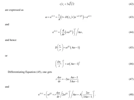
r r < (42)

are expressed as

( ) 1

(

₍

₎

( )2

)

( )

e r 1 D r r_s e r e r

A

ν µ µ

ω_{= = +} − ₌

(43)

and

( ) d

(

1 2

)

2

e ,

d

r

r A

r

λ  _ω  _ω

= _ _ (44)

and hence

(

)

1 2 1

s r

D A

r ω ω

  = −

 

  (45)

or

(

)

2

2 1

s Dr

A

r ω ω

 _{ = −}

 

  (46)

Differentiating Equation (45), one gets

d 1

2

d 3 1

A r

r A

ω _ω ω

ω − = −

− (47)

and

( ) 1 2 d 1 2 2 2 2

e 2 .

d 3 1

r

r A A

r A

λ _ω ω _{ω ω} ω

ω

 

 

=_ + _ = _{ }

−

    (48)

Imposing the continuity of the asymptotic expression, Equation (31) and the non-asymptotic expression, Equ-ation (45) at

(

r rs,ω =

)

(

3 3 2 ,1 3

)

(49)

one gets

2 3.

A= D+ (50)

The most appropriate region in the parameter space is

3 and 0,

A> D> (51)

[image:6.595.69.540.80.432.2]

since the range of coordinate, r, is covered by the origin and the positivity of the metric functions are main-tained.

Figure 1 showes the picture of g₀₀ =eν( )r =

ω

as a function of r r_s , namely the picture of the gravitational potential with the shift of the y axis and a scale factor of 2.

In the region of Equation (51), the distance r can be reached at zero when

ω

reaches ∞, as

2 3

.

s Dr Ar

ω _{= } _

  (52)

Notice that there is an undecided one parameter which can be fixed for the physics inside the horizon at

3 3

2.6 .

2 s s

1 2 3 4 5 6 7 8 9 10 0.1

0.2 0.3 0.4 0.5 0.6 0.7 0.8 0.9 1.0

Figure 1. The metric function, g00

( )

r , as a funtion of r rs in the SSS physical metric.

7. Time Delay Experiment by a Black Hole

If a time delay experiment of a binary pulsar is performed by a black hole companion, one needs a higher order correction of gravity. From Equation (31) and Equation (33), one gets

(

)

(

)

2 3 2

2 1

d

.

dr rs 3 1

ω ω

ω

ω

− =

− (54)

Then, using Equation (14) and Equation (34) one gets

(

)

(

)

(

)

2

2 2

0 0

1

d d d

1

d d

d _{1 1}

s r

t t

r r

ω ω

ω

ω ω ω ω ω

−

= = −

− − (55)

and hence the time delay is expressed as

(

)

(

)

(

)(

)(

)

0

1 2 0 0

0 2

1 d

, 1

s r

t ω

ω

ω ω ω

ω ω ω ω ω ω

ω ω + −

−

∆ = − − −

−

∫

(56)

where ω₀ is the time metric function at the impact parameter r₀,

( )

( )

0 r0 g00 r0 ,

ω =ω = (57)

0 0 0 3

1 2 1

4

ω± = −ω ± ω  − ω 

  (58)

Outside of the horizon,

0 1 3,

ω ω≥ > (59)

and the time delay ∆t is peaked logarithmically at ω₀ as is in the case of Shapiro experiment,

(

)

2 2 2 2

0 0

dr r −r =ln r+ r −r .

∫

(60)

However, when one reaches at the horizon

0 1 3,

ω = (61)

one gets

1 3

ω₋ = (62)

and

4 3.

ω₊ = (63)

Then, the integration of ∆t diverges, since the two zeros inside the squre root coincide. In other words, the time delay at the horizon become infinity. This is an important characteristic of the time delay of black hole companion of a binary pulsar.

This divergence property may be related with the characteristic of the physical metric, in which the horizon,

3 3 , 2

s r

r= (64)

is, at the same time, a circular radius. This is because the speed of light in the radial direction vanishes at the ho-rizon,

d 0, d

r

t = (65)

while the speed of light in the spherical direction is that in vacuum for the physical metric.

8. The Other Experimental Tests of General Relativity

The other tests of General Relativity are shown to be insensitive to the presence of the c₁ term. For the bend-ing of light, one uses the formula,

( ) ( )2 2 ( ) 2 ( ) 2

d

e e e

d

r r r r

r J r

r

µ λ ν µ

φ _{= ±} − + − ₋ −

(66)

(

)

(

)

0 1 1 1

2 2

0 0 0 0 0

1

1 .

2 2 2

s

r b a r c r

r

r r r r r r r r

r r r

    

 

= ± _ + _ − + _ − __+ _

+ +

−     

(67)

Integrating this from a large distance, one gets the well-known expression for the bending of light [2],

(

1 1

)

0 0

2 .

s s

r r

b a

r r

φ

∆ = − = (68)

The integration of the c₁ term in Equation (67) gives a vanishingly small value and therefore this term is in-sensitive to the value of c₁, as is seen from Equation (68) [7].

( ) ( )2 2 ( ) 2 ( ) 2

d

e e e

d

r r r r

r J r E

r

µ λ ν µ

φ _{= ±} − + − ₋ − ₋

(69)

1 2

1 1

1 2

1 1 1 1

1 2

1 1 1 1

s

r b a r r

a c

r a r r r r r

r

r r r r

+ ⋅

+ ⋅ + ⋅

⋅ +

    +   

= ± _ + _ + − +  +  + − _+ _

 ₋  ₋       

  

  

 (70)

where r± are the semi major and minor axis of the elliptical orbit. The appearance of a2 is necessitated by the cancellation of the lowest term for the determination of the constants J2 and E J2. Integration over the el-lipse yields the advancement of perihelion,

2

1 1 1

1

π 1 1 2

2 .

2

s

r a

b a c

r r a

φ

+ −

  

∆ = _ + _ − + + _

   (71)

Due to the relationship, Equation (7), 2 1

1 2

0 a c

a

+ = , one obtains [2]

(

1 1

)

π 1 1 3π 1 1

2 .

2 2

s s

r r

b a

r r r r

φ

+ − + −

   

∆ = _ + _ − = _ + _

    (72)

It is remarkable that the c₁ term and a₂ term cancel each other and the final result is again independent of

1

c [7]. In other words, both equations, Equation (68) and Equation (72), which have been supported by obser-vational data, are insensitive to the value of c₁. The reason for these phenomena is that the bending of light and the advancement of perihelia are variations in the angular variables, which are less ambiguous coordinates. On the other hand, the time delay experiment, Equation (16), formally depends on the parameter c₁. Notice that from Equation (38) in the physical metric,

1 1 1

a =c = − (73)

and

2

1 , 2

a = − (74)

one can see that the relationship

2 1

1 2

0 a c

a

+ = (75)

is automatically satisfied.

For the gravitational red shift and the gravitational lensing, one uses the first order of gravity in g₀₀

( )

r ,

( )

00 1 s .

g r = −r r (76)

Then, both metrics, the Schwarzschild metric and the physical metric, give the same prediction for the all ex-periments in this section at the present time. However, if future exex-periments find the higher order effects, such as the gravitational red shift near or inside black holes, then these observations will substantiate the difference between the both metrics. In fact, the gravitational shift inside the horizon in the physical metric is shown to be gravitationally blue shifted.

9. Summary and Discussion

bigger than the Schwarzschild radius and the gravity inside the horizon shows a repulsive force. Some of these properties will be tested by the observations of the MIT Haystack Observatory. The author has demonstrated that the change of the metric shows the direction of general relativity and points to a new way of understanding the nature of gravity.

Acknowledgements

It is a great pleasure to thank Peter K. Tomozawa, Malia M. Tomozawa and Tai N. Tomozawa for reading the manuscript.

References

[1] Misner, C.W., Thorne, K.S. and Wheeler, J.A. (1973) Gravitation. Freeman, San Francisco.

[2] Weinberg, S. (1972) Gravitation and Cosmology. Wiley and Sons, New York.

[3] Shapiro, I.I., et al. (1966) Physical Review Letters, 17, 933. http://dx.doi.org/10.1103/PhysRevLett.17.933

Resenberg, R.D. and Shapiro, I.I. (1979) Astrophysical Journal, 234, L219. http://dx.doi.org/10.1086/183144

[4] Bertotti, B., Iess, L. and Tortora, P. (2003) Nature, 425, 374. http://dx.doi.org/10.1038/nature01997

[5] Schwarzschild, K. (1916) Sitzungsber. Press. Skad. Wiss. Berlin Math. Phys, 189-196. [6] Jacoby, B.A., et al. (2003) Astrophysical Journal, 599, L99. http://dx.doi.org/10.1086/381260

Demorest, P.B., et al. (2010) Nature, 467, 1087. http://dx.doi.org/10.1038/nature09466

[7] Duff, M.J. (1974) DRG, 5, 441.

Appendix: The Schwarzschild Solution

Setting

( )

eµr =1, (77)

in Equation (1), and using the Maple program the Einstein Equation reads

( )

_e ( )r _{1 0,}

rλ′ r λ

− − + = (78)

( )

( )

e r 1 0

rν′ r λ

− + − = (79)

and

( )

( )

( )

( )

2

( ) ( )

2ν′ r −2λ′ r +2rν′′ r +rν′ r −rν′ r λ′ r =0. (80)

From the sum of Equation (78) and Equation (79), one gets

( )

r

( )

r 0.

ν′ +λ′ = (81)

Using this relation, Equation (80) becomes

( )

( )

2

( )

2 0

rλ′′ r rλ′ r λ′ r

− + − = (82)

or equivalently

( )

(

( )

)

eλr re−λr ′′ =0. (83)

On the other hand, Equation (78) can be written as

( )

(

re−λr

)

′ =1, (84) which solution is

( )

e r 1 B,

r λ

− _{= +}

(85)

and Equation (83) is satisfied, where B is an integration constant. The solution of Equation (81) reads

( ) 1

e r 1 B .

A r

ν ₌  ₊ 

 

  (86)

The asymptotic solution with the boundary condition is given by

1, s.

A= B= −r (87)

On the other hand, the non-asymptotic solution is given by

, Aarbiray.

s

B=Dr (88)