Phonetic Feature Discovery in Speech using Snap Drift

University of East London Institutional Repository: http://roar.uel.ac.uk

This paper is made available online in accordance with publisher policies. Please scroll down to view the document itself. Please refer to the repository record for this item and our policy information available from the repository home page for further information.

To see the final version of this paper please visit the publisher’s website. Access to the published version may require a subscription.

Author(s):

Lee, Sin Wee; Palmer-Brown, Dominic.

Article title:

Phonetic Feature Discovery in Speech using Snap-Drift

Year of publication:

2006

Citation:

Lee, S. W. and Palmer-Brown, D. (2006). "Phonetic Feature Discovery in Speech using Snap-Drift." International Conference on Artificial Neural Networks (ICANN'2006) (Athen, Greece, 10th - 14th September 2006), S. Kollias et al. (Eds.): ICANN 2006, Part II, LNCS 4132, pp. 952 -962.

Link to published version:

http://dx.doi.org/10.1007/11840930_99

Learning

 

Sin Wee Lee and Dominic Palmer­Brown 

Innovative Informatics Research Group  http://www.uel.ac.uk/scot/ii/index.htm  University of East London, Essex, Rm8 2AS, UK 

{SinWee, D.Palmer­Brown}@uel.ac.uk 

Abstract. This paper presents a new application of the snap­drift algorithm [1]:  feature  discovery  and  clustering  of  speech  waveforms  from  non­stammering  and stammering speakers. The learning algorithm is an unsupervised version of  snap­drift  which  employs  the  complementary  concepts  of  fast,  minimalist  learning  (snap)  &  slow  drift  (towards  the  input  pattern)  learning.  The  Snap­  Drift  Neural  Network  (SDNN)  is  toggled  between  snap  and  drift  modes  on  successive  epochs.  The  speech  waveforms  are  drawn  from  a  phonetically  annotated  corpus,  which  facilitates  phonetic  interpretation  of  the  classes  of  patterns discovered by the SDNN. 

1 

Introduction

 

Stuttering (stammering) is a highly  variable condition which occurs across ages and  cultures.  There  is  a  lack  of  consensus  in  establishing  the  criteria  for  a  definition.  Finding a way of identifying exactly what phonetic characteristics are associated with  stammering,  as  opposed  to  non­stammering  speech,  has  proved  elusive.  Perceptual  analysis  is  known  to  be  compromised  by  its  subjectivity  [2],  [3].  In  contrast,  a  correlative  data  analysis  to  characterise  the  acoustic  properties  of  stammering  is  realisable.  There  are  four  classes  of  sound  pressure  wave  that  form  the  acoustic  structure  of utterances  [4]:  Periodic  ‘voice’:  regular repeating  fluctuations  produced  by vocal fold vibration; Aperiodic ‘noise’: ongoing irregular fluctuations in voiceless  fricatives;  Transient  ‘burst’:  brief  irregular  fluctuations  as  in  voiceless  plosives;  or  Silent: no acoustic energy is emitted. The speech sounds used in human languages are  made up of combinations of the four categories. 

The  snap­drift  learning  algorithm  first  emerged  as  an  attempt  to  overcome  the  limitations  of  ART  learning  in  non­stationary  environments  where  self­organisation  needs to take account of periodic or occasional performance feedback. Since then, the  snap­drift  algorithm  has  proved  invaluable  for  continuous  learning  in  several  applications. 

of reinforcement, has been used in the analysis and interpretation of data representing  interactions between trainee network managers and a simulated network management  system [7]. New patterns of the user behaviour were discovered. 

The further exploration ofsnap­drift, in the form of a classifier [8] has been used in  attempting to discover and recognize phrases extracted from Lancaster Parsed Corpus  (LPC)  [9].  Comparisons  carried  out  between  snap­drift  and  MLP  with  back­  propagation, show that the former is faster and just as effective. 

This paper describes the further exploration of snap­drift, in unsupervised form, in  attempting  to  discover  the  defining  and  unique  millisecond  features  in  the  speech  patterns,  which  will  be  used  to  help  understand  the  language  learning  of  non­  stammering and stammering speakers. 

2 

The Snap­Drift Neural Network (SDNN) Architecture

 

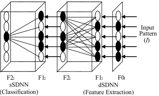
[image:3.595.173.428.377.531.2]

The  modular  neural  network  modified  from  the  Performance­guided  Adaptive  Resonance Theory (P­ART) network, first introduced by Lee & Palmer­Brown [1] is  shown in Fig. 1. 

Fig. 1. SDNN Architecture 

On  presentation  of  an  input  pattern  at  the  input  layer  F01,  dSDNN  will  learn  to  group the input patterns according to their general features. In this case, 10 F21 nodes,  whose  weight  prototypes  best  match  the  current  input  pattern,  are  used  as  the  input  data  to  the  sSDNN  module  for  feature  classification.  In  both  of  the  modules,  the  standard matching and reset mechanism of ART [5], [6] is discarded. Instead, in the  dSDNN module, the output nodes  with the highest net input are always accepted as  winners. In the sSDNN module, a quality assurance threshold is introduced. If the net  input  of  a  sSDNN  node  is  above  the  threshold,  the  output  node  is  accepted  as  the  winner, otherwise a new uncommitted output node will be selected as the new winner  and initialised with the current input pattern. 

Input  Pattern 

(I) 

F22  F12  F21  F11  F01  dSDNN  (Feature Extraction)  sSDNN 

In this version of SDNN we introduce weight re­initialisation.  The main purpose  of  weight re­initialisation  is  to  enable  unused  output  nodes  to  be  reinstated  into  the  competition for winning nodes. Weight re­initialization is invoked after many epochs  since the SDNN must first allow input patterns to settle into their categories. After a  duration defined by a certain number of input patterns, called a learning era (an era is  a number  of  epochs),  the  weights  of nodes  unused  during  the preceding  era  will  be  reinitialised to enable them to participate again in the competition for the best winning  nodes.  In  effect,  reinitialisation  is  a  neuron  pruning  algorithm.  It  removes  weight  vectors that are redundant. 

The following is a summary of the steps that occur in SDNN: 

Step 1: Initialise parameters: (a = 1, s = 0), era =  2000 

Step 2: For each epoch (t) 

Test: Weights re­initialization condition  For each input pattern 

Step 2.1:  Find the D (D = 10) winning nodes at F21 

with the largest net input 

Step 2.2: Inhibit the F21 node for weights re­ 

initialization 

Step 2.3:  Weights of dSDNN adapted according to the 

alternative learning procedure: (a,s) 

becomes Inverse(a,s) after every successive  epoch 

Step 3: Process the output pattern of F21 as input 

pattern of F12 

Step 3.1: Find the node at F12 with the largest net 

input 

Step 3.2: Test the threshold condition: 

IF (the net input of the node is greater than the  threshold) 

THEN 

Weights of the sSDNN output node adapted according  to the alternative learning procedure: (a,s) 

becomes inverse (a,s) after every successive epoch  ELSE 

An uncommitted sSDNN output node is selected and  its weights are adapted according to the 

alternative learning procedure: (a,s) becomes  Inverse(a,s) after every successive epoch 

Weights re­initialization condition: 

After ‘era’ input patterns 

IF (F21 node not used for the past era input 

Re­initialize the F21 node with randomly selected input 

pattern 

Inhibit the F21 node for weights re­initialization for 

the next era input pattern presentation  ELSE 

No action taken. 

3 

The Snap­Drift Algorithm

 

The  learning  algorithm  combines  a  modified  form  of  Adaptive  Resonance  Theory  (snap) [10] and Learning Vector Quantisation (drift) [11]. In general terms, the snap­  drift algorithm can be stated as: 

Snap­drift=a(Fast_Learning_ART) +s(LVQ)  (1)  The top­down learning of both of the modules in the neural system is as follows: 

wJi (new) = a(I ÇwJi (old) ) +s(wJi (old) +b (I ­ wJi (old) ))  (2)  where wJi = top­down weights vectors; I = binary input vectors,  and b  = the drift  speed constant = 0.5. 

In  successive  learning  epochs,  the  learning  is  toggled  between  the  two  modes  of  learning.  When a  =  1,  fast,  minimalist  (snap)  learning  is  invoked,  causing  the  top­  down  weights  to  reach  their  new  asymptote  on  each  input  presentation.  (2)  is  simplified as: 

wJi (new) = I ÇwJi (old)  (3)  This learns sub­features of patterns. In contrast, when s= 1, (2) simplifies to: 

wJi (new) = wJi (old) +b (I ­ wJi (old) )  (4)  which causes a simple form of clustering at a speed determined byb. 

The  bottom­up  learning  of  the  neural  system  is  a  normalised  version  of  the  top­  down learning. 

wiJ (new) = wJi (new) / | wJi (new) |  (5)  where wiJ (new) = top­down weights of the network after learning. 

In SDNN, as described in section 2, snap­drift is toggled between snap and drift on  each successive epoch. The effect of this is to capture the strongest clusters (holistic  features), sub­features, and combinations of the two. 

4 

Simulations

 

simulations, pre­processing of the utterances is completed. In this research, each point  of  a  speech  utterance  waveform  collected  represents  1  ms  of  speech  data.  In  this  research, in order to analyze and recognise the acoustic properties of the speaker with  sufficient  precision,  each  utterance  is  sampled  every  10  points  for  a  total  of  1000  points,  which  represents  about  1  second  of  speech  information.  This  is  considered  sufficient  by  a  phonetics  expert.  Figure  2  shows  the  example  of  sampled  utterance  used in the simulations. Each of the sampled waveforms is used to generate a number  of input patterns for SDNN. The input patterns are generated using a sliding window  of size 100 samples points. The sliding window is shifted to the right by 25 sample  points to create a new input. This provides some  overlapping of  features among the  input  patterns.  Then,  each  input  pattern  is  converted  into  a  1400  bit  coarse  coded  binary  pattern.  5  utterances  are  used  from  2  speakers,  3  utterances  from  the  non­  stammering speaker and 2 from the stammering speaker. Table 1 shows the range and  properties  of  the  input  set,  making  the  total  number  of  input  patterns,  1873  input  vectors. These test input patterns are presented in sequence to SDNN. The number of  input patterns for each speaker varies because: 

1.  Each speaker is asked to speak using different types of statements. 

2.  Non­stammering speaker will produce more fluent speech utterances with shorter  or no delay between phrases. 

3.  Stammering  speakers  always  produce  longer  utterances  due  to  the  delay  in  the  voiceless fricative. 

The  input  patterns,  which  are  also  quite  noisy,  provide  a  real  world  test  for  unsupervised SDNN as a feature discovery and classification system. 

[image:6.595.201.396.533.606.2]

For SDNN to act as a viable classifier, and to demonstrate the utility of the features  it acquires,  it  should  be  able  to  estimate  or  predict  whether  a  speaker  in a real­time  scenario  is  non­stammering  or  stammering  when  a  speech  utterance  is  fed  into  the  system. An estimation will be made of how long it takes to be certain that a speaker is  non­stammering or stammering. 

Table 1.  Range and properties of the input set 

Speaker group  Total number of Inputs  Non­stammering  256 

­40000  ­30000  ­20000  ­10000  0  10000  20000  30000  40000 

[image:7.595.195.422.158.262.2]

1  516 1031 1546 2061 2576 3091 36064121 4636 5151 5666 6181 

Fig. 2.  Example utterance waveform used in simulation 

4.1  Results 

[image:7.595.124.478.432.552.2]

The results are presented in Table 2 to Table 4; each of the tables shows the example  category  types  formed  by  the  SDNN  network  with  their  acoustic  properties.  The  acoustic  properties  record  is  obtained  from  a  phonetics  expert’s  annotation  of  the  speech  waveform  corpus.  Each  of  the  sampled  sequence  of  the  speech  utterance  is  identified  with  one  or  more  acoustic  properties:  Silent,  Periodic,  Aperiodic  and  Transient. 

Table 2. Accoustic properties of example category type 1 (Stammering) 

Input  Speaker group  Silent  Periodic  Aperiodic  Transient 

195  Non­stammering  ü ü ü

211  Non­stammering  ü ü

377, 456  Stammering  ü

432, 68  Stammering  ü ü

473, 485, 575,  585 

Stammering 

ü

570  Stammering  ü ü

595  Stammering  ü ü

609  Stammering  ü ü

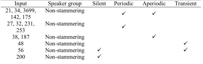
Table 3.  Accoustic properties of example category type 2 (Non­Stammering) 

Input  Speaker group  Silent  Periodic  Aperiodic  Transient  21, 34, 3699, 

142, 175 

Non­stammering  _{ü ü}

27, 32, 231,  253 

Non­stammering 

ü

38, 187  Non­stammering  ü

48  Non­stammering  ü

56  Non­stammering  ü ü

[image:7.595.123.474.582.693.2]

304  Stammering  ü ü ü

[image:8.595.123.473.201.320.2]

310  Stammering  ü ü

Table 4.  Accoustic properties of example category type 3 (Mixture of both type of speakers) 

Input  Speaker group  Silent  Periodic  Aperiodic  Transient  45, 108  Non­stammering  ü ü

165  Non­stammering  ü

131, 135  Non­stammering  ü ü

204, 123  Non­stammering  ü

283, 504  Stammering  ü ü

304, 442  Stammering  ü ü ü

615, 565, 370,  457 

Stammering 

ü

546, 547  Stammering  ü

By looking at the tables, it is clear that the SDNN has categorised the input patterns  into 3 distinctive types, stammering speech, non­stammering speech, and a category  type with a mixture of the two speaker types. The three category types were identified  since they corresponded to different non­overlapping sets of sSDNN output nodes. 

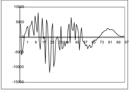
Fig. 3.Example input waveform for category type 1 (Input 377) 

­15000  ­10000  ­5000  0  5000  10000 

[image:8.595.209.420.391.537.2]

[image:9.595.218.415.161.308.2]

Fig. 4.Example input waveform for category type 1 (Input 595) 

Fig.  3  ­  5  show  the  example  input  waveforms  being  grouped  into  the  same  category,  in  this  case  example  category  type  1  (Stammering).    By  comparing  these  waveforms, the similarities can be easily identified. In order to understand the learned  features of the speech utterances, a comparison of the input patterns of the system and  the learned weight templates is performed. 

[image:9.595.200.408.516.662.2]

The input patterns received by the SDNN are binary coarse coded representations  of the fragments of speech input utterances, such as those shown in Fig. 3 – 5. Each  point  in  the  speech  input  is  represented  by  a  14  bit  binary  representation.  So,  the  weights learned are the results of processing these binary input patterns. As a means  of visualization, the weights learned are thresholded as a first order approximation to  produce a binary representation of the weights learned. Then, the 14 bit coarse binary  representation  of  the  weights  learned  are  decoded  to  show  the  actual  waveform  features that have been acquired from the original waveforms. 

Fig. 5.Example input waveform for category type 1 (Input 456) 

­8000  ­6000  ­4000  ­2000  0  2000  4000  6000 

1  9  17  25  33  41  49  57  65  73  81  89  97  ­3000 

­2000  ­1000  0  1000  2000  3000 

[image:10.595.197.415.151.296.2]

Fig. 6.  Example weights learned for category type 1 (Winning node 42) 

­4000  ­3000  ­2000  ­1000  0  1000  2000  3000  4000 

1  8  15 22  29  36  43  50 57  64  71  78  85  92  99 

Fig.7.Example weights learned for category type 1 (Winning node 13) 

Fig.  6  and  Fig.  7  show  the  weights  learned.  Although  these  weights  graphs  are  drawn using approximation for visualization, the figures clearly show that system has  learned the features in the input patterns of the categories. In fig. 6 and 7, the graphs  show a noisy sinusoid of about 3  Hz. By comparing with the original waveforms, it  has  clearly  shown  that  what  these  waveforms  have  in  common  is  a  sinusoid  of  approximately  3Hz.  The  phonetics  expert  has  identified  that  these  parts  of  the  utterances  are  often  associated  with  silence  or  pauses  or  gaps  between  words  where  there is some sound perhaps but no clear articulation. This is indeed known to be the  case for stammerers. 

­4000  ­3000  ­2000  ­1000  0  1000  2000  3000  4000 

[image:10.595.201.407.338.486.2]

5 

Unique Sequences and Classifications

 

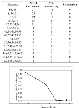
As  mentioned,  during  each  learning  epoch,  the  speech  utterances  are  fed  into  the  system in sequence, one speaker utterance at a time. In order to do the analysis and  thus  determine  the  time  it  takes  to  identify  the  speaker  type,  one  epoch  after  convergence  is  randomly  selected.  By  randomly  selecting  one  sequence  of  sSDNN  winning  nodes  to  start  with,  the  whole  epoch  is  examined  to  find  any  repeated  occurrences of the sequence. These repeated occurrences of winning nodes sequences  are called unique sequences if they are unique to only stammering or non­stammering  speakers.  Then,  the  speaker  input  utterances  which  caused  the  unique  sequence,  is  examined.  With  this  method  of  analysis,  the  length  of  unique  sequence  of  winning  nodes  which  only  occurred  in  a  particular  group  of  speakers,  either  stammering  or  non­stammering, will determine the time the system takes to be certain of the speaker  group for a particular speech utterance. 

Table  4  shows  the  sequence  occurrence  of  winning nodes  for  non­stammering  or  stammering  group  input  patterns. The  sequences  for  analysis  are randomly  selected.  In the table, most of the sequences with the length less than 3 tend to have a mixture  of  occurrence  of  both  types  of  speaker  groups.  By  increasing  the  length  of  the  sequence, some form of bias arises. With the sequence length of more than 5 winning  nodes, these sequences only occur in one of the speaker types, either non­stammering  or  stammering.  For  example,  the  sequence  {45,  52,  43,  19,  65}  only  exists  in  the  speech  input  of  the  stammering  speaker.  Obviously,  this  sequence  is  unique  to  the  stammering  speaker.  By  plotting  the  average  ratio  of  the  speaker  type  over  the  sequence  length,  the length  of  the  sequence  which  can  be  labelled  as  unique  can  be  identified. This is illustrated in Fig. 3. In fig. 3, the average ratio of the speaker group  for sequence length of 5 and 6 is the lowest. With this number of randomly selected  sequences  for  consideration,  it  confidently  shows  that  input  patterns  for  particular  speaker  groups  can  be  identified  when  a  unique  sequence,  with  the  length  of  5  winning nodes is used for analysis. 

By identifying this unique sequence; we mean SDNN is capable of identifying the  speaker group of input patterns after system convergence is achieved. As mentioned  in  section  IV,  each  input  pattern  roughly  represents  about  1  second  of  speech  information, thus, SDNN is capable of distinguishing the type of speaker by analysis  of about 5 seconds of speech, which is analogous to the a person identifying a speaker  as stammering or non­stammering after hearing several words. Since not all words are  stammered by stammerers, this figure is also of the order of 5 seconds of speech for  humans. 

0.00  0.20  0.40  0.60  0.80  1.00  1.20  1.40  1.60 

2  3  4  5  6 

[image:12.595.158.435.198.577.2]

Sequence length  Av e ra g e  ratio o f sp e a k e r t y p e s  

[image:12.595.160.435.201.577.2]

Table 5. Randomly selected sequence occurrence of winning nodes for non­stammering /  stammering group input patterns 

Fig. 7.  The average ratio of the speaker type over the length of the winning node sequence 

6 

Conclusion

 

This paper presents the new application of feature discovery in phonetics speech data  using the snap­drift algorithm. It also gives the opportunity to test the performance of  SDNN  without  performance  feedback  in  a  purely  unsupervised  mode.  SDNN  categorizes  the  input  patterns  according  to  their  general  and  distinct  features.  By 

Sequence  No. of  Occurrences 

Non­ 

stammering  Stammering 

63, 65  21  13  9 

1, 36, 31  25  9  6 

7,5,3  19  11  8 

45,52,43  15  6  9 

12,23,34,34  11  6  7 

7,5,3,54,39  4  4  0 

42,34,46,10,59  3  3  0 

45,52,43,19,65  7  0  7 

7,7,2,6,49  3  3  0 

39,36,56,16,32  4  0  4 

6,32,40,4,23,58  6  1  5 

69,68,56,68,69  3  0  3 

54,69,55,11,46,50  3  0  3  11,63,45,37,56,68  4  4  0 

examining the phonetic and waveform properties of the input patterns in each of the  categories  formed,  it  has  been  shown  that  without  any  performance  feedback,  the  SDNN  modules  group  the  input  patterns  sensibly  and  extract  properties  which  are  general between non­stammering and stammering speech, as well as distinct features  within each of the utterance groups, thus supporting classification. 

References

 

[1]  Lee, S. W., Palmer­Brown, D., Roadknight, C. M.: Performance­guided Neural Network for Rapidly  Self­Organising Active Network Management. Neurocomputing, Vol. 61C (2004) 5 – 20. 

[2]  Aylett, M., Turk, A.: Vowel Quality in Spontaneous Speech: What makes a good vowel. Proc. of Int.  Conf. of Spoken Language Processing. Sydney, Australia. 

[3]  Klatt, D. H.: Review of Text­to­Speech Conversion for English. Online collection (1987)  [4]  Ladefoged, P.: A Course in Phonetics. 4th ed., Boston, Heinle & Heinle (2001) 

[5]  Lee,  S.  W.,  Palmer­Brown,  D.,  Tepper,  J.,  Roadknight,  C.  M.:  Snap­Drift:  Real­time  Performance­  guided Learning. Proc. of IJCNN, Portland, Oregon, Vo1. 2 (2003) 1412 – 1416. 

[6]  Lee,  S.  W.,  Palmer­Brown,  D.,  Roadknight,  C.  M.:  Reinforced  Snap­Drift  Learning  for  Proxylet  Selection in Active Computer Networks. Proc. of IJCNN, Budapest, Hungary, Vo1. 2 (2004) 1545 –  1550. 

[7]  Donelan,  H.,  Pattinson,  C.,  Palmer­Brown,  D.,  Lee,  S.  W.:  The  Analysis  of  Network  Manager’s  Behaviour  using  a  Self­Organising  Neural  Networks.  Proc.  of  ESM,  Magdeburg,  Germany,  (2004)  111 – 116.. 

[8]  Lee, S. W., Palmer­Brown, D.: Phrase Recognition using Snap‑Drift Learning Algorithm. Proc.  of IJCNN, Montreal, Canada (2005). 

[9]  Garside,  R.,  Leech,  G.,  Varadi,  T.:  Manual  of  Information  to  Accompany  the  Lancaster  Parsed  Corpus: Department of English, University of Oslo (1987). 

[10]  Carpenter,  G.  A.,  Grossberg,  S.:  A  Massively  Parallel  Architecture  for  a  Self­Organising  Neural  Pattern Recognition Machine. Com. Vision, Graphics and Image Proc., Vol. 37 (1987) 54­115.  [11]  Kohonen,  T.:  Improved  Versions  of  Learning  Vector  Quantization.  Proc.  of  IJCNN,  Vol.  1  (1990)