Study of Stability Analysis for a Class of Fourth Order Boundary Value Problems

http://dx.doi.org/10.4236/am.2014.513182

Study of Stability Analysis for a Class of

Fourth Order Boundary Value Problems

C. Bala Rama Krishna1_{, P. S. Rama Chandra Rao}2

1_{Department of Mathematics, Chaitanya Degree College (Autonomous), Warangal, India} 2_{Department of Mathematics, Kakatiya Institute of Technology & Science, Warangal, India}

Email: [email protected], [email protected]

Received 16 April 2014; revised 28 May 2014; accepted 8 June 2014

Copyright © 2014 by authors and Scientific Research Publishing Inc.

This work is licensed under the Creative Commons Attribution International License (CC BY). http://creativecommons.org/licenses/by/4.0/

Abstract

Fourth order differential equations are considered to develop the class of methods for the numer-ical solution of boundary value problems. In this paper, we have discussed the regions of absolute stability of fourth order boundary value problems. Methods proposed and derived in this paper are applied to solve a fourth-order boundary value problem. Numerical results are given to illu-strate the efficiency of our methods and compared with exact solution.

Keywords

Numerical Differentiation, Initial Value Problem, Boundary Value Problem, Absolute Stability, Multistep Methods

1. Introduction

The determination process for the numerical solution of initial value problems in ordinary differential equations can be classified into two categories-single step methods and multistep methods. Single step methods are those in which the approximation for the point x=xn+1 involves information from only one of the previous points

n

x=x . Methods using the approximation at more than one previous points to determine the approximation at the next point are called multistep methods. Thus a k-step method requires information about the solution at k points x xn, n−1,,xn k− +1 to compute the solution at the point xn+1. Finite difference methods for boundary value

has considered high order stiffly stable methods. Further information can be had from [7] and [8]. Special multistep methods based on numerical differentiation for solving the initial value problem have been derived in Rama Chandra Rao [9]. The methods now to be discussed are based on replacing the function f x y x

(

,

( )

)

which is unknown, by an interpolating polynomial having the values f_n = f x y

(

_n, _n

)

on a set of points xn where yn has already been computed. The methods discussed in this paper are essentially based on the idea that the so-lution is best approximated by polynomials. The motivation for the work carried out in this paper arises from the methods based on numerical differentiation for the first-order differential equations, special multistep methods based on numerical integration for the solution of the special second-order differential equations by Henrici [5] and Special multistep methods based on numerical differentiation for solving the initial value problem by Rama Chandra Rao [9]. In Henrici [5] methods based on Numerical Integration have been derived by integrating

( )

,

y′′ = f x y twice and replacing the function f x y

( )

, by an interpolating polynomial. Special multistep me-thods have been derived by replacing y x

( )

on the left hand side ofyiv

( )

x = f x y

( )

, by an interpolating po-lynomial and differentiating it four times. We have investigated a class of implicit methods. It is found that the implicit methods have order

(

k−3

)

. Some local truncation errors are provided. The regions of absolute stabili-ty of the methods are derived. Numerical tests of the performance of the methods are established by solving dif-ferential equation and compared with the exact solution. The numerical results reported show the validity of our methods.

2. General Linear Multistep Methods for Special Fourth-Order Differential

Equations

The special fourth order differential equation

(

,

) ( )

, 0 0,

( )

0 0,

( )

0 0,

( )

0 0

iv

y = f x y y = y y′ =y′ y′′ = y′′ y′′′ = y′′′ (1)

occurs frequently in many number of problems of science and engineering.

A general linear multistep method of step number k for the numerical solution of equation (1) is given by

4

1 1 1 0 1

k k

n j j n j j j n j

y+ =

∑

=a y + − +h

∑

= b y+ − (2)

where aj, bj are constants and “h” is the step length. Introducing the polynomials

( )

1

( )

1

1 and 1

k k

k k k

j j

j a j b

ρ ξ ξ ξ − σ ξ ξ −

= =

= −

∑

=

∑

(3)

Equation (2) can be written as

( )

4

( )

1 1 0

iv

n k n k

E y h E y

ρ − + − σ − + = (4)

In Equation (4), “E” is the shift operator defined by E y

( )

n = yn+1

Applying (4) to yiv=λy, we get the characteristic equation

( )

( )

4

whe , re 0

h h h

ρ ξ − σ ξ = =λ (5)

The roots ξi of the characteristic Equation (5) and h are in general, complex and the region of absolute stability is defined to be the region of the complex h -plane such that the roots of the characteristic Equation (5) lie within the unit circle whenever h lies in the interior of the region. Denoting the region of absolute stability of R and its boundary by ∂R, the locus of ∂R is given by

( )

( ) ( )

ei ei , 0 2π

h θ =ρ θ σ θ ≤ ≤θ (6)

3. Derivation of the Methods

Let p x

( )

be the backward difference interpolating polynomial of y x

( )

at

(

k+1

)

abscissas xn+1,xn,,xn k− +1.

Then p x

( )

is given by

( )

( )

(

1

)

1

0 1 ,

m m n

n k

m

x x

s

p x y s

m h + + = − −   = − _{ }∇ =  

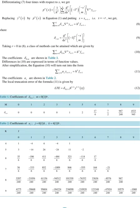
Differentiating (7) four times with respect to x, we get

( )

4 44

( )

1

0

1 d

1 .

d k

iv m m

n m

s

p x y

m

h = s +

 −   

=_{  } − _{ }∇  

∑

  

Replacing yiv

( )

x by piv

( )

x in Equation (1) and putting x=xn+ −1 r i.e. s= −r, we get,

4

, 1 1

0

m

r m n n r

m k

y h f

δ _{+ + −}

= ∇ =

∑

(8)

where

( )

4 , 4 d 1 d m r m s m s

δ = _ − _− _  

  (9) Taking r = 0 in (8), a class of methods can be attained which are given by

4

0, 1 1

0

m

m n n

m k

y h f

δ _{+ +}

= ∇ =

∑

(10)

The coefficients δ0,m are shown inTable 1.

Differences in (10) are expressed in terms of function values. After simplification, the Equation (10) will turn out into the form

4

1 1

0 k

j n j n

j= a y+ − =h f +

∑

(11)

The coefficients aj are shown inTable 2.

The local truncation error of the formula (11) is given by

( )

1 1

0, 1

k k k

[image:3.595.90.539.85.754.2]

LTE=δ ₊h + y + η (12)

Table 1. Coefficients of δ_0,m; m=0 1 9

( )

.

M 0 1 2 3 4 5 6 7 8 9

0,m

δ 0 0 0 0 1 2 17

[image:3.595.87.537.351.720.2]

6 7 2 967 240 4523 945

Table 2. Coefficients of aj; j=0 1

( )

k, k=4 1 9

( )

.

K J

0 1 2 3 4 5 6 7 8 9

4 1 −4 6 −4 1

5 3 −14 26 −24 11 −2

6 35

6 186 6 − 411 6 484 6 − 321 6 114 6 − 17 6

7 56

6 333 6 − 852 6 1009 6 − 846 6 555 6 − 164 6 21 6 −

8 3207

240 21056 240 − 61156 240 94512 240 − 101530 240 76352 240 − 33636 240 8576 240 − 967 240

9 4275

It follows that the k-step method (14) has the order k−3, which is absolutely stable for h∈ −

[

4, 0

]

For the method (13), we have

( )

0 and

( )

k k j k

j j a

ρ ξ ξ − σ ξ ξ

=

=

∑

= . (13)

The regions of absolute stability of the method for k = 4, 5, 6, 7, 8 and 9 are shown inFigure 1 andFigure 2

[image:4.595.122.505.186.706.2]

(Taking real part on x-axis and imaginary part on y-axis). The region of absolute stability is the region lying out-side the boundary.

Figure 1. The region of absolute stability of the method (13) for k = 4, 5 and 6.

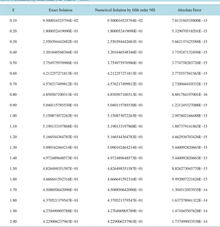
4. Numerical Example

In this section, we have applied ND methods to solve the differential equation

( )

( )

( )

( )

sin , 0 0, 0 1, 0 1, 0 0

iv

y = +y x y = y′ = y′′ = − y′′′ = (14)

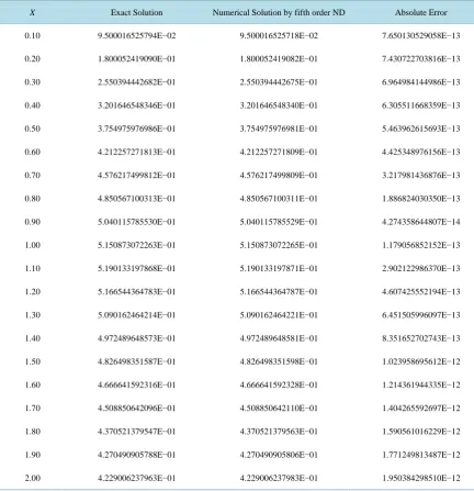
in the interval

[ ]

0, 4 with h = 0.01 and h = 0.02 and the results are shown inTable 3 andTable 4. The fourth order numerical differentiation method derived in this paper for k = 6 is

4

1 1 2 3 4 5 1

186 411 484 321 114 17 6

35 35 35 35 35 35 35

n n n n n n n n

y+ = y − y− + y− − y− + y− − y− + h f + (15)

5. Discussion and Conclusion

[image:5.595.92.535.261.717.2]

The methods based on numerical integration are found to be closed regions of absolute stability; the methods

Table 3. Solution by fifth order ND with h = 0.01.

X Exact Solution Numerical Solution by fifth order ND Absolute Error

0.10 9.500016525794E−02 9.500016525794E−02 7.813194535800E−15

0.20 1.800052419090E−01 1.800052419090E−01 5.329070518201E−15

0.30 2.550394442682E−01 2.550394442681E−01 5.662137425588E−15

0.40 3.201646548346E−01 3.201646548346E−01 3.719247132494E−15

0.50 3.754975976986E−01 3.754975976986E−01 3.774758283726E−15

0.60 4.212257271813E−01 4.212257271813E−01 2.775557561563E−15

0.70 4.576217499812E−01 4.576217499812E−01 2.720046410332E−15

0.80 4.850567100313E−01 4.850567100313E−01 8.881784197001E−16

0.90 5.040115785530E−01 5.040115785530E−01 1.221245327088E−15

1.00 5.150873072263E−01 5.150873072263E−01 2.997602166488E−15

1.10 5.190133197868E−01 5.190133197868E−01 1.887379141863E−15

1.20 5.166544364783E−01 5.166544364783E−01 4.662936703426E−15

1.30 5.090162464214E−01 5.090162464214E−01 5.440092820663E−15

1.40 4.972489648573E−01 4.972489648573E−01 5.440092820663E−15

1.50 4.826498351587E−01 4.826498351587E−01 8.826273045770E−15

1.60 4.666641592316E−01 4.666641592316E−01 9.992007221626E−15

1.70 4.508850642096E−01 4.508850642096E−01 1.304512053935E−14

1.80 4.370521379547E−01 4.370521379547E−01 1.637578961322E−14

1.90 4.270490905788E−01 4.270490905789E−01 1.471045507628E−14

[image:6.595.89.522.101.549.2]

Table 4. Solution by fifth order ND with h = 0.02.

X Exact Solution Numerical Solution by fifth order ND Absolute Error

0.10 9.500016525794E−02 9.500016525718E−02 7.650130529058E−13

0.20 1.800052419090E−01 1.800052419082E−01 7.430722703816E−13

0.30 2.550394442682E−01 2.550394442675E−01 6.964984144986E−13

0.40 3.201646548346E−01 3.201646548340E−01 6.305511668359E−13

0.50 3.754975976986E−01 3.754975976981E−01 5.463962615693E−13

0.60 4.212257271813E−01 4.212257271809E−01 4.425348976156E−13

0.70 4.576217499812E−01 4.576217499809E−01 3.217981436876E−13

0.80 4.850567100313E−01 4.850567100311E−01 1.886824030350E−13

0.90 5.040115785530E−01 5.040115785529E−01 4.274358644807E−14

1.00 5.150873072263E−01 5.150873072265E−01 1.179056852152E−13

1.10 5.190133197868E−01 5.190133197871E−01 2.902122986370E−13

1.20 5.166544364783E−01 5.166544364787E−01 4.607425552194E−13

1.30 5.090162464214E−01 5.090162464221E−01 6.451505996097E−13

1.40 4.972489648573E−01 4.972489648581E−01 8.351652702743E−13

1.50 4.826498351587E−01 4.826498351598E−01 1.023958695612E−12

1.60 4.666641592316E−01 4.666641592328E−01 1.214361944335E−12

1.70 4.508850642096E−01 4.508850642110E−01 1.404265592697E−12

1.80 4.370521379547E−01 4.370521379563E−01 1.590561016229E−12

1.90 4.270490905788E−01 4.270490905806E−01 1.771249813487E−12

2.00 4.229006237963E−01 4.229006237983E−01 1.950384298510E−12

based on numerical differentiation are found to be absolutely stable outside some closed boundaries. We have obtained the solution by numerical differentiation methods which are derived in this paper and are more accurate. The absolute errors are very small.

References

[1] Bala Rama Krishna, C., Rama Chandra Rao, P.S., Vishwa Prasad Rao, S. and Nageswara Rao, B. (2013) Finite Dif-ference Methods for the Solution of a Class of Singular Perturbation Problems. International Journal of Mathematical Sciences and Engineering Applications, 7, 411-421

[2] Eskandari, Z. and Dahaghin, M.S. (2012) A Special Linear Multi Step Method for Special Second Order Differenial Equations. International Journal of Pure and Applied Mathematics, 78, 1-8.

[3] Gear, C.W. (1971) Numerical Initial Value Problems in Ordinary Differential Equations. Prentice Hall,Upper Saddle River.

188-209.http://dx.doi.org/10.1145/321217.321223

[5] Henrici, P. (1962) Discrete Variable Methods in Ordinary Differential Equations. Wiley, New York. [6] Jain, M.K. (1984) Numerical Solution of Differential Equations. Wiley Eastern Ltd.,New Delhi.

[7] Kalyani, P. and Rama Chandra Rao, P.S. (2013) Solution of Boundary Value Problems by Approaching Spline Tech-niques. International Journal of Engineering Mathematics, 2013, Article ID: 482050.

[8] Kalyani, P. and Rama Chandra Rao, P.S. (2013) A Conventional Approach for the Solution of the Fifth Order Bound-ary Value Problems Using Sixth Degree Spline Functions. Applied Mathematics, 2013, 583-588.

currently publishing more than 200 open access, online, peer-reviewed journals covering a wide range of academic disciplines. SCIRP serves the worldwide academic communities and contributes to the progress and application of science with its publication.