Statistical Classification Using the Maximum Function

http://dx.doi.org/10.4236/ojs.2015.57068

Statistical Classification Using the Maximum

Function

T. Pham-Gia1_{, Nguyen D. Nhat}2_{, Nguyen V. Phong}3

1_{Université de Moncton, Moncton, Canada}

2_{University of Economics and Law, Hochiminh City, Vietnam} 3_{University of Finance and Marketing, Hochiminh City, VietNam}

Received 8 October 2015; accepted 14 December 2015; published 17 December 2015

Copyright © 2015 by authors and Scientific Research Publishing Inc.

This work is licensed under the Creative Commons Attribution International License (CC BY). http://creativecommons.org/licenses/by/4.0/

Abstract

The maximum of k numerical functions defined on p

R , p≥1, by f_max

( )

x =max

{

f₁

( )

x ,,f_k

( )

x

}

,

p x R

∀ ∈ is used here in Statistical classification. Previously, it has been used in Statistical Dis-crimination [1] and in Clustering [2]. We present first some theoretical results on this function, and then its application in classification using a computer program we have developed. This ap-proach leads to clear decisions, even in cases where the extension to several classes of Fisher’s li-near discriminant function fails to be effective.

Keywords

Maximum, Discriminant Function, Pattern Classification, Normal Distribution, Bayes Error, L1-Norm, Linear, Quadratic, Space Curves

1. Introduction

In our two previous articles [1] and [2], it is shown that the maximum function can be used to introduce new ap-proaches in Discrimination Analysis and in Clustering. The present article, which completes the series on the uses of that function, applies the same concept to develop a new approach in classification that can be shown to be versatile and quite efficient.

Baye-sian Decision Theory approach starts with the determination of normal (or non-normal) distributions fi

go-verning these data sets, and also prior probabilities qi (with sum 1 1

C i i=q =

∑

) assigned to these distributions. More general considerations include the cost ci j of misclassifications, but since in applications we rarely

know the values of these costs they are frequently ignored. We will call this approach the common Bayesian one. Here, the comparison of the related posterior probabilities of these classes, also called “class conditional distribu-tion funcdistribu-tions”, is equivalent to compare the values of gi =q fi i, and a new data point x0 will be classified into

the distribution gi₀ with highest value of gi

( )

x0 , i.e. i₀

( )

0 max

{

j

( )

0

}

j

g x = g x .

On the other hand, Fisher’s solution to the classification problem is based on a different approach and remains an interesting and important method. Although the case of two classes is quite clear for the application of Fish-er’s linear discriminant function, the argument and especially the computations, become much harder when we are in the presence of more than two classes.

At present, the multinormal model occupies, and rightly so, a position of choice in discriminant analysis, and various approaches using this model have led to the same results. We have, in Rp, p≥1

( )

( )

( ) 1( )

1 2 1 2 2 1 e , 2π p p f R − ′ − − −

= x x ∈

x Σ x

Σ

µ µ

(1)

1) For discrimination and classification into one of the two classes, we have the two equations:

( )

( )

( )

( ) 1( )

1 2 1 2

2 e , 1, 2,

2π

i i i

i

i i i p

i q

g q f i

− ′

− − −

= = x x =

x x Σ

Σ

µ µ

and their ratio g1

( ) ( )

x g2 x =q f1 1

( )

x q f2 2

( )

x , supposing the cost of misclassification can be ignored.

2) In general, using the logarithm of g x

( )

we have:

( )

( )

1

(

)

1

(

)

1

(

)

ln ln 2π ln ln .

2 2

i gi i i i p i qi

φ _{= = − −} ′ − _{− − + +}

x x x µ Σ x µ Σ (2)

Expanding the quadratic form, we obtain:

( )

i i i i

φ x =xA x′+B x C′ + ,

where

1 1

2 , ,

i i i i i

− −

= − =

A Σ B Σ µ and 1

(

1 _{ln 2}π ln

)

_{ln .}

2

i i i i p i qi

− _′

= − + + +

C µΣ µ Σ (3)

This function φi

( )

x is called the quadratic discriminant function of class πi, by which we will assign a

new observation to class πi₀ when φi0

( )

x0 has the highest value among all φi

( )

x0 . Ignoring Ai,

( )

i i i

θ x =B x C′ + is called the linear discriminant function of class i. We will essentially use this result in our approach.

An equivalent approach considers the ratio of two of these functions

( )

( ) ( )

1,2 φ1 φ2

∆ x = x x (4)

and leads to the decision of classifying a new observation as in class π1 if this ratio is larger than 1.

The presentation of our article is as follows: in Section 2, we recall the classical discriminant function in the two-class case when training samples are used. Section 3 formalizes the notion of classification and recalls sev-eral important results presented in our two previous publications, which are useful to the present one. Section 4 presents the intersections of two normal surfaces and their projections on Oxy. Section 5 deals with classifica-tion into one of C classes, with C>2. Fisher’s approach for multilinear classification is briefly presented there, together with some advantages of our approach. In Section 6, we present an example in classification with

4

C= , solved with our software Hammax. The minimum function is studied in Section 7 while Section 8 presents the non-parametric approach, as well as the non-normal case, proving the versatility of Hammax.

2. Classification Rules Using Training Samples

variances and obtain the following results: 1) Σ1=Σ2 =Σ using

*

S and xi,i=1, 2 The decision rule is then:

For a new vector x0, allocate it to class π1 if

(

)

( )

_* 1

(

)

( )

_* 1

(

)

1 2 0 1 2 1 2

1 1 ln 2 q q − −  −  ′ ′ − − − + _{≥  }  

x x S x x x S x x , (5)

and to class π2, otherwise. Here *

S is the estimate of the common variance matrix Σ, and can be obtained by pooling S1 and S2.

We can see that the discriminant function ld x

( )

is linear in x, since

( ) (

)

( )

1

* 1 2

−

′

= − −

ld x x x S x A, (6)

where

(

)

( )

* 1

(

)

1 2 1 2

1 2

−

′

= − − +

A x x S x x and x0∈π1 if ld x

( )

0 ≥0.

2) Different covariance matrices: Σ1≠Σ2

For a new vector x0, we consider the quadratic discriminate function qd x

( )

, and allocate it to π1 if

( )

1 1 1 1

0 1 1 2 2 0 0 1 2 0

1 1 ln 2 q k q − − − −  −   ′ ′  ′  =_ − _ − _ − _{ − ≥  }  

qd x x S x S x x S S x , (7)

and to π2, otherwise, where

(

)

(

1 1

)

1 2 1 1 1 2 2 2

ln . 2 k − − ′ ′ + −

= S S x S x x S x

3. Classification Functions

3.1. Decision Surfaces and Decision Regions

Let a population consist of C disjoint classes. We now present our approach and prove that for the two class case it coincides with the method in the previous section.

Definition 1. A decision surface D x

( )

is a surface defined in Rp+1 that separates points assigned to a specific class, from those assigned to other classes.

Definition 2. Let

{

}

1

C

i i i _i

g =q f ₌ be a finite family of densities

{ }

1

C i _i

f ₌ , with prior weights

{ }

1

C i _i

q ₌ , with

( )

{

( )

( )

}

max max 1 , , ,

p C

g x = g x  g x x∈R .

A max-classification function _{{ }}

i

g

ϕ is a mapping from a domain Ω ⊂Rp into the discrete family

{

1, 2,,C

}

, defined as follows:

For a value x0∈ Ω, ϕ{ }gi

( )

x0 =i0, s.t. gi0

( )

x0 =gmax

( )

x0 . 3.2. Properties of gmax(⋅)

There are several other properties associated with the max function and we invite the reader to look at these two articles [2] and [1], to find:

1) Clustering of densities using the width of successive clusters. L1-distance between 2 densities is well-known but does not apply when there are more than 2 densities. Let us consider k densities

( )

, 1, , ,

i

f x i=  k with k≥3 and let

( )

{

( ) ( )

( )

}

max max 1 , 2 , , ,

p k

f x = f x f x  f x ∀ ∈x R .

A L1-distance between all densities taken at the same time, cannot really be defined, and the closest to it is a weighted sum of pairwise L1-distances. However, using fmax, we can devise a measure which could be

( )

1, 2, , k 1 _Rp max d 1

f f  f ≡

∫

f x x−

and is slightly different than the case k=2. We have the double inequality

1 2 1

1 1

max _{i j} 2 , , , _{k i j}

i j _{i j}

f f f f f f f

< − ≤  ≤

∑∑

− .

2) Considering now gmax =max

{ }

gi , we study the basic properties of gmax, and its role as a classifier.

Sev-eral original results related to L1-distances, overlapping coefficients and Bayes errors, are established, for two and more densities. This error can be shown to be 1−

∫

gmax

( )

x dx and several applications were presented.

From [6] and [7], we have the double inequality

{

₁

}

{ }

max

( )

₁

1 1

max min d 1 ,

2 i j i j i i Rp i j

i j

g g q g g g

k <

 

− + ≤ ≤  − + 



∑∑



∫

x x

with Bayes error given by

( )

_{( )}

_{( )}

1,2, , max

1 1

1 p d , , ,

q

k _R

Pe g q

C C

 

  _{= − = } 



 

∫

x x

 

since p _max

( )

d

R g

∫

x x still represents the unconditional probability of correct classification.

4. Discrimination between 2 Classes

For simplicity and for graphing purpose we will consider only the bivariate case p=2 in the rest of the article. However, all arguments can be applied to the case p>2, and the basic answer on the classification of a new data point is still provided.

4.1. Determining the Function gmax

Our approach is to determine the function gmax and use it with the max-classification function φ{ }g_i . This is

achieved by finding the regions of definition of gmax in 2

R , i.e. by determining their boundaries as projections onto the horizontal plane of intersections between transformed normal surfaces

{

_,

( )

}

3

i

x g x ∈R , and the value of

{

x g, max

}

there.

1) For the two-class case we show that this approach is equivalent to the common Bayesian approach recalled earlier in Section 2. First, from Equation (6), equation ld x

( )

=0 determines precisely the linear boundary of the two adjacent regions where gmax =qf1 and gmax = −

(

1 q f

)

2 respectively, and hence the two approaches

are equivalent in this case. Second, from Equation (7), qd x

( )

=0 also determines the quadratic boundary (ies) of the region separating gmax =qf1 from gmax = −

(

1 q f

)

2 since the two surfaces g1 and g2 intersect each

other along curves which have quadratic projections (Straight lines, Ellipses, Parabolas or Hyperbolas) on the horizontal plane. But whereas the common Bayesian approach only retains only the linear, or quadratic, boun-dary for decision purpose, gmax retains a partial surface on each side of the boundary and atop of the horizontal

plane. This fact makes the max-classification function much more useful.

When the dimension of p exceeds 2 we have these projections as hyperquadrics, which are harder to visualize and represent graphically.

2) For the C classes case, C>2: In general, when there are C classes the intersections between each of the

2 C

   

  couples of normal surfaces

{ }

fi are space curves in

3

R , and their projections into the horizontal plane

determine definition regions of fmax.

These regions are given below. Once they are determined they are clearly marked down as assigned to class i, or to class j, and the family of all these regions will give the classification regions for all observations. Naturally, definition regions for gmax are deformations of those of fmax, but have to be computed separately since there is

no rules to go from one set of regions to the other. They are identical only in the case q1 =q2 = ⋅⋅⋅ =qC =1C.

4.2. Intersections of Normal Surfaces

Below are some examples for the normal case.

Two normal surfaces, representing f1 and f2, always intersect each other along a curve, or two curves in 3

R , which, when projected in the (x, y)-plane, give(s) a quadratic curve, whose equation can be obtained by solving f1= f2, where

( )

( )

( ) 1( )

1 2 1 2 2

1

e , 1, 2

2π i i i p i f i − ′ − − −

= x x =

x Σ

Σ

µ µ

.

In R2, taking the logarithm, we have:

( )

(

)

2 2 2 2 1

ln , 2

2 1

1

ln , 1, 2.

2π 1

i i i i

i i i i

i i

x x y y

i i

x x y y

i

x y i

x x y y

f x y

i

µ µ µ µ

ρ

σ σ σ σ

ρ

σ σ ρ

_{ −   −  −   − }    = − _ _ − _ _  _{ }+ _   − _{       }     + =  ₋   

Equaling the two expressions we obtain equations of the projections (in the horizontal plane) of the intersec-tions curves in R3. There are several cases for these intersections, depending on the values of the mean vectors and the covariance matrices. We do not give them here, to avoid confusion, but they are sketched in the appen-dix and are available upon request. Instead, we give clear examples and graphs of the different cases.

1) A straight line (when covariance matrices are equal), or a pair of straight lines, parallel or intersecting each other.

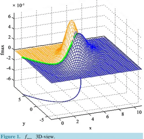
2) A parabola: This happens when µ1≠µ2 and σx1σx2 and σy1 σy2. Example 1.

Let 1

5.00 1.43

 

=  

 

µ , 2

4.58 2.97

 

=  

 

µ , 1

2 2 2 5

 

=  

 

Σ , 2

1 1 1 4

 

=  

 

[image:5.595.157.467.142.271.2] [image:5.595.190.440.476.717.2]

Σ and ρ1=0.6325,ρ2=0.5.

Figure 1 shows the graph of max

{

f f1, 2

}

in 3D where the intersection of these two normal surfaces is a

parabola.

max

f ’s boundary: The equation of this parabola is

2

0.5x 2.85x 1.3066y 4.4 0

− + + − =

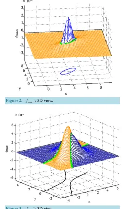
3) An ellipse: When µ1=µ2, and ρ1=ρ2.

Example 2.

Let 1 2

4 4

 

= _{=  }

 

µ µ , 1

0.3525 0.2714 0.2714 0.3790

 

=  

 

Σ , 2

2.2031 1.6962 1.6962 2.3687

 

=  

 

Σ , ρ1=ρ2=0.7425 , (σx2 =2.5σx1

[image:6.595.83.529.57.736.2]

and σy₂ =2.5σy₁).

Figure 2 shows the graph of max

{

f f1, 2

}

in 3D, where the intersection of these two normal surfaces is an

ellipse.

The equation of this ellipse is

2 2

5.3114x −7.6069y +4.94xy−12.0634x−9.0923y+38.6461 0=

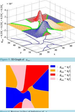
4) A hyperbola: This happens when µ1≠µ2 and σx1 ≠σx2, σy1 ≠σy2.

Example 3. Let 1

1.5 1.0

 

=  

 

µ , 1

1.80 0.27 0.27 1.00

 

=  

 

Σ , ρ =1 0.16, 2

1.0 1.0

 

=  

 

µ , 2

3.00 1.45 1.45 1.00

 

=  

 

Σ , ρ =2 0.84.

[image:6.595.182.434.284.714.2]

Figure 3 shows the graph of max

{

f f1, 2

}

in 3D, where the intersection of these two normal surfaces is a

Figure 2. f_max’s 3D view.

hyperbola.

The equation of this hyperbola is

2 2

0.562x 3.049y 2.3702xy 2.4957x 1.8133y 1.3936 0.

− + − − + + =

5. Classification into One of C Classes (C

≥

3)

The gmax function is quite simple when the three class covariance matrices are equal, as can be seen from

Fig-ure 4(a). Then the discriminant functions are all straight lines intersecting at a common point. These lines are projections of normal surface intersection curves.

In the case these matrices are unequal they can intersect according to a complicated pattern, as shown in Fig-ure 4(b).

5.1. Our Approach

For normal surfaces of different means and covariance matrices, in the common Bayesian approach we can use (6) or (7), or equivalently, classify a new value x0 into the class j0 such that φj0

( )

x0 =max_j

{

φj

( )

x0

}

. In the common Bayesian approach, we have the choice between:

1) One against all, using the

(

C−1

)

discriminant functions (6), with the dichotomous decision each time:

0

x is in group j or not in group j.

2) Two at a time, using C C

(

−1 2

)

expressions (6) or (7) with regions delimited by straight lines or qua-dratic curves, each expression classifies new data as in Ci or Cj.

As pointed out by Fukunaga ([8], p. 171) these methods can lead to regions not clearly assignable to any group. In our approach, we use the second method and compile all results so that R2 is now divided into disjoint sub-regions, each having a surface atop of it, which constitute the graph of gmax in

3

R . Then, for a new ob-servation x0, to classify it we just use the max-classification function ϕ{ }g_i given in Definition 2.

5.2. Fisher’s Approach

It is the method suggested first [9], in the statistical literature for discrimination and then for classification. It is still a very useful method. The main idea is to find, and use, a space of lesser dimensions in which the data is projected, with their projections exhibiting more discrimination, and being easier to handle.

1) Case of 2 classes. It can be summarized as follows:

2, 2, 1 1

C= p= r= − =p : Projection into a direction which gives the best discrimination: Decomposition of total variation

,

T = W+ B

S S S

with SW =S1+S2 and

(

)(

)

, i

i i i

D

∈

′

=

∑

− −

x

S x m x m 1

k i

i k

D i

n ∈

=

∑

x

m x , i=1, 2. We then search for a direction

w such that

( )

1 22

2 2 1 2

m m

J

s s

− =

+

w  

 

is maximum, where mi and

2

i

s are projected values into that direction. We have W1

(

1 2

)

−

= −

w S m m with

(

1 2

)(

1 2

)

B= − − ′

S m m m m .

Fisher’s method in this case reduces to the common Baysian method if we suppose the populations normal. Implicitly it already supposes the variances equal. But Fisher’s method allows the consideration that variables can be can enter individually, so as to measure their relative influence, as in analysis of variance and regression.

2) Fisher’s multilinear method (extension of the above approach due to CR Rao): C classes, of dimension p and r= − <C 1 p.

Projection into space of dimr: Decomposition of total variation in original space:

(

)(

)

T = − − ′

x

S Σ x m x m , 1 Ci ₁ni i

n =

=

∑

(a)

[image:8.595.94.536.81.692.2]

(b)

(

)(

)

1 i

C

W i= ∈D i i

′

=

∑ ∑

_x − −

S x m x m ,

(

)(

)

1 .

C

B i=ni i i

′

=

∑

− −

S m m m m

The projection from a p-dim space to a

(

C−1

)

-dim space is done with a matrix W and we have y=W x′ . Using y, let the projected quantities be SW =W S W′W , SB =W S W′ B . We want to find the matrix W so

that the ratio J

( )

W = SB SW is maximum. Solving SB−λiSW =0 to obtain λi and then solving

(

S_B−λ_iS_W

)

w_i=0 to have eigenvectors wi, we obtain the matrix W , which often is not unique. Within the

(

C−1

)

-dim space a probability distribution can be found for the projected data, which will provide cut-off val-ues to classify a new observation into one of the C classes.

We can see that Fisher’s multilinear method can be quite complicated.

5.3. Advantages of Our Approach

Our computer-based approach offers the following advantages: 1) It uses concepts at the base: Max of

{ }

1

C i i

g ₌ , and is self-explanatory in simple cases. It avoids several ma-trix transformations and projections of Fisher’s method, which could, or could not be done.

2) The determination of the maximum function is essentially machine-oriented, and can often save the analyst from performing complex matrix or analytic manipulations. This point is of particular interest when this analysis concerns vectors of high dimensions. To classify a new observation x0 into the appropriate group, say j0, it

suffices now to find the index j0 so that gj₀

( )

x0 =gmax

( )

x0 . This operation can always be done since C is

finite.

3) Complex cases arise when there are a large number of classes, or a large number of variables (high value for p). But as long as the normal surfaces can be determined the software Hammax can be used. In the case where p is much larger than the sample sizes, we have to find the most significant dimensions and use them only, before applying the software.

4) It offers a visual tool very useful to the analyst when p=2. The full use of the function g_max in 3

R necessitates the drawing of its graph, which could be a complex operation in the past, but not now. In general, the determination of the intersections between densities (or between gi) in

1

p

R + , and their projections into

p

R , gives more insights into the problem: in classical statistical discriminant analysis, we only deal with these projections, and do not consider the curves in Rp, of which they are projections (Equation (6) and Equation (7)). Hence, for any other family of densities which has the same intersections in Rp as those already consi-dered, we would have the same classification rule. For p≥3 integration of gmax is carried out using an

ap-propriate approach (see [1]) and classification of a new data point can again be made.

5) Regions not clearly assignable to any group, are removed with the use of gmax, as already mentioned.

6) For the non-normal case, gmax can still provide a simple practical approach to classification, as can be

seen in Example 6, where gmax does allow us to derive classification rules. [10] can be consulted for this case.

7) It permits the computation of the Bayes error, which can be used as a criterion in ordering different classi-fication approaches. Naturally, the error computed by our software from data is an estimation of the theoretical, but unknown, Bayes error obtained from population distributions.

6. Output of Software Hammax in the Case of 4 Classes

The integrated computer software developed by our group is able to handle most of the computations, simula-tions and graphic features presented in this article. This software extends and generalizes some existing routines, for example the Matlab function Bayes Gauss ([5], p. 493), which is based on the same decision principles.

Below are some of its outputs, first in the case of classification into a four-class population.

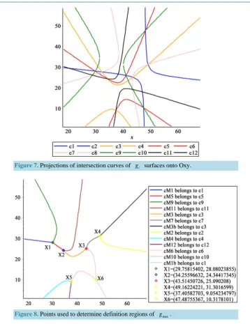
Example 4. Numerical and graphical results determining gmax in the case of four classes in two dimensions 1, 2, 3, 4

f f f f , i.e. Xi ~N

(

µi,Σi

)

,i=1, 2, 3, 4, with

1 2 3 4

40 48 43 38

, , ,

20 24 32 28

X = _{ } X = _{ } X = _{ } X = _{ }

1 2

35 18 28 20

,

18 20 20 25

S =_ _ S =_ − _

−

   ,

3 4

15 25 5 10

,

25 65 10 70

S =_ _ S =_ − _

−

   

{

}

max max 1 1, 2 2, 3 3, 4 4

g = q f q f q f q f , where q1=0.25,q2=0.20,q3=0.40,q4=0.15. Figure 5 gives the 3D

graph of gmax in Oxyz (with projections of the intersection curves onto Oxy):

To obtain Figure 6 we use all intersection curves given in Figure 7 below.

In this example we have all hyperbolas as boundaries in the horizontal plane. Their intersections will serve to determine the regions of definition of gmax. Figure 8 below shows us these regions.

Classification: For the new observation, for example (25, 35), we can see that it is classified in C4.

Note: In the above graph, for computation purpose we only consider gmax within a window [ , ] [ , ]a b × c d in

Oxy, with a=18.06, b=61.94, c=3.32, d =56.68. We can show that outside this window the values of the integrals of q f1 1,,q f4 4 are negligible and using these results we can compute

∫

_R2gmax

( )

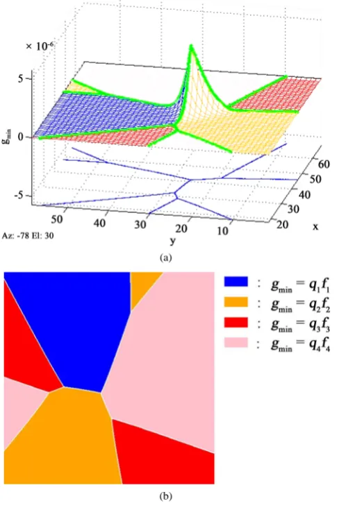
x dx=0.7699.

7. Risk and the Minimum Function

[image:10.595.221.361.87.150.2]

1) When risk, as the penalty in misclassification, is considered in decision making we aim at the min risk ra-ther than the max risk. In the literature, to simplify the process, we usually take the average risk, also called Bayes

Figure 5. 3D Graph of g_max.

[image:10.595.181.440.329.712.2]

[image:11.595.132.491.75.541.2] [image:11.595.152.474.323.532.2]

Figure 7. Projections of intersection curves of g_i surfaces onto Oxy.

Figure 8. Points used to determine definition regions of gmax.

risk, or the min of all max values of all different risks, according to the minimax principle.

We suppose here that risk Ri has fi as its normal probability distribution, function of 2 variables x and y,

and various competing risks

{ }

1

C k k

R ₌ are present.

A minimum-classification function _{{ }}

(

,

)

i

g x y

ψ is defined similarly to _{{ }}

(

,

)

i

g x y

φ .

Definition 4. A min-classification function _{{ }}

i g

ψ is a mapping from a domain Ω ⊂Rp into the discrete family

{

1, 2,,C

}

, defined as follows:

For a value x0∈ Ω, ψ{ }gi

( )

x0 =i0, s.t. gi0

( )

x0 =gmin

( )

x0 .

2) A relation between the max and min functions can be established by using the inclusion-exclusion prin-ciple:

(

)

(

)

( )

1

(

)

max 1 min , min , , 1 min 1, , .

k k

i i j i j l k

i i j i j l

f =

∑

₌ f −

∑

_< f f +

∑

_{< <} f f f + ⋅⋅⋅ + − − f  f

subgroups of

{ }

fi Ci=₁. For classification purpose we classify a new set of data

(

x y0, 0

)

as belonging to the

class having the lowest risk at that point. The function gmin represents the minimum risk, but is, however, the

invisible part of the graphs since it lies below all surfaces gi.

Example 5. The four normal distributions are the same as in Example 1 but represent the densities of the risks associated with the problem. Using the same prior probabilities the function gmin is given by Figure 9(a)

while its definition regions are given by Figure 9(b).

For gmin, similarly to gmax, we can approximately compute

∫

gmin

( )

x dx=0.007546.

Remarks: a)For the two-population case this integral is also the overlap coefficient and can be used for infe-rences on the similarity, or difference between the two populations.

b) The boundaries between regions defining gmax are in general linear or quadratic curves coming from the

intersections of normal surfaces. Boundary between regions defining gmin can be simpler since they might not

come from these intersections.

8. Applications and Other Considerations

8.1. The Software Hammax

This software has been developed by our research group and is part of a more elaborate software to deal with discrimination, classification and cluster analysis, as well as with other applications related to the multinormal distribution. This software is in further development to be interactive and more user-friendly, and has its own

(a)

[image:12.595.193.436.337.705.2]

(b)

copyright. It will also have more connections with social sciences applications.

8.2. The Non-Parametric Density Estimation Approach

A more general approach would directly use data available in each group to estimate the density of its distribu-tion. The gmax function approach to classification would then follow, exactly as for the normal case. But,

un-less we approximate the density obtained by parametric methods, different regions of definition of gmax can

only be obtained empirically, to be used in the classification of a new data x0. Densities of all classes are now

estimated by the classical kernel density estimation method for two variables, x1 and x2. Using the kernel

( )

1 2

exp 2 2π

t

K t = _− _

 ,

they are estimated by

(

)

1

1 1 2 2

1 2

0

1 2 1 2

ˆ ˆ

1

, , 1, , ,

n

j j

i

j

x x x x

f x x K K i C

nh h h h

−

=

  −   − 

 

=      =

    

 

∑



where

(

xˆ1j,xˆ2j

)

is the j-th observation. Optimal values for h1 and h2 has been discussed by various authors

([11]). We refer to [1] where a numerical example was redone, using density estimation. Also, we have the as-sociated function g*max. The Bayes error

( )

_{( )}

2

1 3 *

1,2 1 _R max d 0.125

Pe  = −

∫

g x x= ,

computed by simulation, gives the same value as for the parametric normal case.

8.3. Non-Normal Model

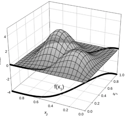
As stated earlier an approach based on the maximum function is valid for non-normal populations. We construct here an example for such a case.

Let us consider the case where the population density f x x1

(

1, 2

)

in

[ ]

2

0,1 , given by

(

)

2

(

)

1 1, 2 i 1 i i; i, i ,

f x x =

∏

₌ h x α β

where h x_i

(

_i;α β_i, _i

)

, i=1, 2, are independent standard beta densities of the first kind, i.e.

(

)

1

(

)

1

(

)

; , i 1 i ,

i i i i i i i i

h x α β =xα− −x β− Beta α β ,

with α β >i, i 0, and 0≤xi ≤1.

Similarly, we have:

(

)

2

(

)

2 1, 2 i 1 i i; i, i ,

f x x =

∏

₌

k

x γ δ

where

k

_i

(

x_i; ,γ δ_{i i}

)

are also independent beta densities.

Example 6. For α =1 3, β =1 6, α =2 4, β =2 7, γ =1 4, δ =1 5 and γ =2 6, δ =2 5 and q=0.35,

the gmax function is defined in

[ ]

2

0,1 by

(

)

{

(

)

(

)

}

max 1, 2 max 0.35 1 1, 2 , 0.65 2 1, 2

g x x = f x x f x x

We can see that the last two functions intersect each other along a curve in

R

3, the projection of which in

2

R is the discriminant curve giving the boundary between the two classification regions, as given by Figure 10, with an equation which is neither linear nor quadratic, since its expression is

( )

(

)

(

)

2 1 1

1 _{2 3} 1

1 1 1

7 1 2

, 0 1,

7 1 2 13

A x x

f x x

A x x Bx

− +

= ≤ ≤

− + +

[image:14.595.211.431.84.279.2]

Figure 10. Two bivariate beta densities, their intersection and its projection.

Any data above the curve, e.g. (0.2, 0.6), is classified as in Class 1. Otherwise, e.g. (0.2, 0.2), it is in Class 2. Numerical integration gives

( )

_{( )}

2 0.35

1,2 1 _R max d 0.1622.

Pe = −

∫

g x x=

9. Conclusion

The maximum function, as presented above, gives another tool to be used in Statistical Classification and Anysis, incorporating discriminant analysis and the computation of Bayes error. In the two-dimensional case, it al-so provides graphs for space curves and surfaces that are very informative. Furthermore, in higher dimensional spaces, it can be very convenient since it is machine oriented, and can free the analyst from complex analytic computations related to the discriminant function. The minimum function is also interested, has many applica-tions of its own, and will be presented in a separate article.

References

[1] Pham-Gia, T., Turkkan, N. and Vovan, T. (2008) Statistical Discrimination Analysis Using the Maximum Function, Communic. in Stat., Computation and Simulation, 37, 320-336. http://dx.doi.org/10.1080/03610910701790475

[2] Vovan, T. and Pham-Gia, T. (2010) Clustering Probability Densities. Journal of Applied Statistics, 37, 1891-1910. [3] Duda, R.O., Hart, P.E. and Stork, D.G. (2001) Pattern Classification. John Wiley and Sons, New York.

[4] Johnson and Wichern (1998) Applied Multivariate Statistical Analysis. 4th Edition, Prentice-Hall, New York.

http://dx.doi.org/10.2307/2533879

[5] Gonzalez, R.C., Woods, R.E. and Eddins, S.L. (2004) Digital Image Processing with Matllab. Prentice-Hall, New York.

[6] Glick, N. (1972) Sample-Based Classification Procedures Derived from Density Estimators. Journal of the American Statistical Association, 67, 116-122. http://dx.doi.org/10.1080/01621459.1972.10481213

[7] Glick, N. (1973) Separation and Probability of Correct Classification among Two or More Distributions. Annals of the Institute of Statistical Mathematics, 25, 373-382. http://dx.doi.org/10.1007/BF02479383

[8] Fukunaga (1990) Introduction to Statistical Pattern Recognition. 2nd Edition, Academic Press, New York. [9] Fisher, R.A. (1936) The Statistical Utilization of Multiple Measurements. Annals of Eugenic, 7, 376-386. [10] Flury, B. and Riedwyl, H. (1988) Multivariate Statistics. Chapman and Hall, New York.

http://dx.doi.org/10.1007/978-94-009-1217-5

[11] Martinez, W.L. and Martinez, A.R. (2002) Computational Statistics Handbook with Matlab. Chapman & Hall/CRC, Boca Raton.

-4 -2 0 2 4

0.0 0.2

0.4 0.6

0.8 1.0

0.0 0.2 0.4 0.6 0.8

gm

ax

x1

x₂

Appendix

In R2, taking the logarithm, we have the equations for a family of quadratic curves:

2 2

11 2 12 22 2 1 2 2 0

a x + a xy+a y + a x+ a y+ =a ,

where,

(

)

(

)

2 1

11 _{2 2 2 2}

2 1

1 1

2 x 1 2 x 1

a

σ ρ σ ρ

= −

− − ,

(

)

(

)

2 1

22 _{2 2 2 2}

2 1

1 1

2 y 1 2 y 1

a

σ ρ σ ρ

= −

− − ,

(

)

(

)

2 2 1 1

2 1

12 _{2 2}

2 1

1 1

x y x y

a ρ ρ

σ σ ρ σ σ ρ

= −

− − ,

(

)

2 2

(

)

1 1

2 2 1 1

2 1

2 1

1 2 2 2 2

2 1

1 1

,

4 1 4 1

x y x y

x y x y

x x

a µ ρ µ µ ρ µ

σ σ σ σ

σ σ

ρ ρ

   

= _− + _− _− + _

− _{ } − _{ }

(

)

22 2 22

(

)

11 1 11

2 1

2 2 2 2 2

2 1

1 1

,

4 1 4 1

y x y x

x y x y

y y

a µ ρ µ µ ρ µ

σ σ σ σ

σ σ

ρ ρ

   

= _− + _− _− + _

− _{ } − _{ }

(

)

2 2 2 2

(

)

1 1 1 1

2 2 1 1

2 2 1 1

2 2

1 1

2 2 2 2

2 1

2 2 2 2

2 2 2 1 2 2 2 1 1 1 2 2

4 1 4 1

1

ln .

1

x y x y x y x y

x y x y

x y x y

x y x y

a µ µ ρ µ µ µ µ ρ µ µ

σ σ σ σ

σ σ σ σ

ρ ρ

σ σ ρ

σ σ ρ

    = _ + − _− _ + − _ − _{ } − _{ }  ₋    −  ₋   