Filtering in Time Frequency Domain using STFrFT

Filtering in Time-Frequency Domain using STFrFT

Pragati Rana

P.G Student Jaypee University of Engineering and Technology,

Guna (India)

Vaibhav Mishra

P.G Student Jaypee University of Engineering and Technology,

Guna (India)

Rahul Pachauri

Sr. Lecturer. Jaypee University of Engineering and Technology,

Guna (India)

ABSTRACT

The Fractional Fourier Transform is a generalized form of Fourier Transform, which can be interpreted as a rotation by angle α in time-frequency plane or decomposition of signals in terms of chirps. However it fails in locating Fractional Fourier Domain Frequency contents. Short-time FRFT variants are suitable for analysis of multicomponent and non-linear chirp signals with improved time-frequency resolution. Short-Time FRFT is the simultaneous representation of, combination of the time and FRFD-frequency information. Filtering in the fractional domain separates the noise and the highly concentrated signal. Filtering results depict that the results in fractional domain give better results. The time-frequency representation in fractional domain is useful tool for various applications like filtering of chirp signals. Simulations are performed on MATLAB platform.

General Terms

Fractional Fourier Transform (FRFT), Shannon Sampling Theorem, Short time Fractional Fourier Transform (STFrFT).

Keywords

Tfd, Stft, Wvd, Stfrft, Frft.

1.

INTRODUCTION

Analysis and processing of non-stationary signals is best done with the help of time-frequency plots, which have got wide range applications including telecommunications, radar, seismic signal analysis, LFM signal analysis and biomedical engineering. Signals with time-variant frequency content are best represented by time-frequency distributions (TFDs) which help to analyze how the energy is distributed over the 2-D time-frequency plane. In Fourier Transform the signal is non-localized with respect to the excluded variable of time whereas in time-frequency distributions the variables t and f are not mutually exclusive, but are present together. The TFD representation is localized in t and f. Analysis of signal in time-frequency domain helps to analyze the properties such as time variation, frequency variation, find number of components, separate the frequency components by filtering in time-frequency domain and for analyzing specific components separately. Several techniques are available to calculate the time-frequency distributions. The Short Time Fourier Transform (STFT) and Wigner-Ville distributions (WVD) are commonly used [1] [2].

1.1 TIME-FREQUENCY DISTRIBUTION

(TFDs):

In order to introduce the time-dependency in Fourier Transform, the spontaneous solution consists of windowing

the signal for a particular time instant, calculate its Fourier Transform and repeat it for the entire length of the signal. STFT is a simple and formidable method which uses the spectrum of a signal segment centered at a time, to represent the instant spectrum of the signal at that time. The results of STFT can be easily inferred and decoded. However, for the chirp signals it has poor resolution. On the other hand other powerful time-frequency representation is WVD which has good resolution as compared to STFT but has fatal disadvantage of producing cross-terms. Cross-terms are produced in the WVD for multi-component signals which make the interpretation of results difficult. Many, methods have been proposed for the cancelation of cross-terms [3]. All these methods are at the cost of time-frequency resolution. The optimized transforms are either poor in resolution or have the problem of cross-term. There is a trade-off between the two quantities.

1.2

CHIRPS

AND

FACTIONAL

FOURIER TRANSFORM:

6

2.

THEORETICAL AND

MATHEMATICAL BACKGROUND:

By multiplying the signal with a window before taking the FrFT, the STFrFT is obtained [7].

𝑆𝑇𝐹𝑟𝐹𝑇𝑥,𝑝 𝑡, 𝑢 = −∞+∞𝑥 𝜏 . 𝑔 𝜏 − 𝑡 . 𝐾𝑝 𝜏, 𝑢 𝑑𝜏 (1)

In order to distinguish it from those with the same window but different order FRFT kernels, it is called the pth order STFrFT in some cases. The window with a short time support is real and symmetric, capturing a portion of the signal around the window center . The FRFT of this portion is viewed as the instantaneous FRFD-spectrum of the signal at instant. By moving the window along axis, the FRFD-spectrum at every instant is obtained. From this 2-D transformation we can see not only the FRFD-frequency contents but also how they change by time. The basis of the STFrFT is denoted by,

ℎ 𝜏 𝑡, 𝑢 = 𝑔 𝜏 − 𝑡 . 𝐾∗ _{𝜏, 𝑢 .}

₍₂₎

The STFrFT in FRFD can be written as,

𝑆𝑇𝐹𝑅𝐹𝑇𝑥,𝑝 𝑡, 𝑢 = _−∞+∞𝑋𝑝 Ɛ . 𝐻𝑝∗ Ɛ 𝑡, 𝑢 𝑑Ɛ

where,

𝐻𝑝 Ɛ 𝑡, 𝑢 = _−∞+∞ℎ 𝜏 𝑡, 𝑢 .𝐾𝑃(𝜏,Ɛ).d𝜏 (4)

= 2П 𝐺((Ɛ-u)csc 𝛼).𝐾𝑝 𝑡, Ɛ . 𝐾−𝑝 𝑡, 𝑢

where, G((Ɛ-u)csc 𝛼) is the scaled, shifted FT of the window g(t).

The time-FRFD-frequency plane is divided by the STFRFT with parallelograms which are called the time-FRFD-frequency cells. The two sides of the time-FRFD-time-FRFD-frequency cell represent the time-width and FRFD-bandwidth that the STFRFT can resolve. Actually, they are the time-width and FRFD-bandwidth of the basis, respectively, which are defined by

𝑇ℎ2 = _{| ℎ 𝜏 𝑡,𝑢 |}1 2 (𝜏 − 𝜏 ℎ)2

+∞

−∞ |ℎ 𝜏 𝑡, 𝑢 |2𝑑𝜏 (5)

𝐵ℎ,𝑝2 = _{| 𝐻} 1

𝑝 𝜀 𝑡,𝑢 |2 (∈ −∈ℎ) 2 +∞

−∞ |𝐻𝑝 ∈ 𝑡, 𝑢 |2𝑑 ∈ (6)

where, mean time and mean FRFD-frequency of the basis are defined as,

𝜏 ℎ= _{| ℎ 𝜏 𝑡,𝑢 |}1 2 𝜏

+∞

−∞ |ℎ 𝜏 𝑡, 𝑢 |2𝑑𝜏 (7)

𝜀 ℎ= _{| 𝐻} 1

𝑝 𝜀 𝑡,𝑢 |2 ∈

+∞

−∞ |𝐻𝑝 ∈ 𝑡, 𝑢 |2𝑑 ∈ (8)

Fig.1: The FRFD-frequency plane divided by time-FRFD-frequency cells

The reciprocal value of the time-FRFD-bandwidth product (TFBP) of the basis is defined as the 2-D resolution of the STFrFT, i.e.

𝑅 = _𝑇 1

ℎ𝐵ℎ ,𝑝

The upper bound of the 2-D resolution of the STFrFT is achieved by Gaussian window and is given by, R = _{sin 𝛼}2

The STFrFT is a windowed FrFT, so its computational complexity depends on that of FrFT. The STFrFT consists of the following number of FrFTs,

𝑂(𝑁𝑙𝑜𝑔2𝑁)

The step size of the moving window is given by N/ƛ , so computational complexity of the STFrFT is given by, 𝑂(𝑁2_𝑙𝑜𝑔

2𝑁)

.

STFrFT can be viewed as a generalized STFT. The STFrFT with order 1 can be termed as the STFT of the signal. The generalized form of FT is FRFT. On similar lines we can say that the generalized form of STFT is STFrFT. STFrFT is also a form of the TFDs, with more concentration due to the fractional domain representation.

3.

FILTERING IN TIME-FREQUENCY

DOMAIN:

The FrFT can be viewed as the generalization of the FT which was introduced by Namias at first and then by Ozaktas [8]. The FrFT can be viewed as the chirp-basis expansion directly from its definition, but essentially it can be interpreted as a rotation in time frequency plane, i.e. unified time-frequency transform. With the order from 0 increasing to 1, the FrFT can show characteristics of signal changing from time domain to frequency domain. The FrFT is most likely to improve the solutions to problems where chirp signals are involved. This is because a chirp signal forms a line in time-frequency plane, and therefore, there exists an order for which such a signal is compact. Chirp signals are not compact in spatial or time domain. Thus, in many such cases, we can filter out the signal easily in an appropriate fractional Fourier domain when it is not possible to separate the signal and noise in space or frequency as shown in figure below:

Fig.2: (a) If filtering is done without rotation signal information is lost. (b) Filtering done after rotation i.e.

after applying FRFT

the signal. The pth _{order (p = 2}

𝛼 / 𝜋

defined as,

𝑋

𝑢 = 𝐹𝑇

𝑥 𝑡 𝑢

₌

_{𝑥 𝑡 . 𝐾}

𝑝

𝑡, 𝑢 . 𝑑𝑡

−∞

where,

𝐾_𝑝 𝑡, 𝑢 = 1−𝑗 cot 𝛼_2𝜋 exp( 𝑗𝑡2+ 𝑢₂ 2 cot 𝛼 − 𝑗𝑢𝑡 csc 𝛼 , 𝛼 ≠ 𝑘𝜋

= δ(u+t) , , 𝛼 = 2𝑘 + 1 𝜋

If chirp rate is known then the signal can be filtered with the matched order. If chirp rate is

𝜇

𝑝

= 2𝛼

/𝜋

𝛼

= cot

(−𝜇

)

𝑥 = exp 𝑗𝜋 0.1 𝑡 + 0.8 3 ₋𝜋 90𝑡

2 _{∗ exp 𝑗𝜋0.4𝑡}2₊

𝑗𝜋6𝑡 ∗ exp⁡(−_10𝑡𝜋2) + exp(j𝜋0.0001𝑡2+ 𝑗𝜋10𝑡) ∗ exp⁡(−_10𝑡𝜋₂).

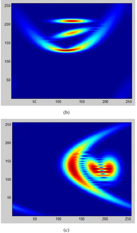
If we consider the STFT of the above signal, it can be defined the STFrFT of the signal with order 1. Consider the spectrograms of the signal with order 1, matched order of the chirp rate and unmatched order of the chirp rate shown below in figure 3(a),(b),(c) respectively. The spectrograms depict that the order of filtering will be decided by the matched order of the STFrFT. The matched order is the necessary condition for filtering the signal in the fractional domain. It can also be seen that the spectrogram or the time-frequency representation of the signal with matched order is crisp and clear. The horizontal axis shows time whereas the vertical axis show the frequency representation of the signal considered. The STFrFT has advantage over the WVD. It removes the cross-term present in WVD. This can be seen in figure 4 (a), (b). The STFrFT is also useful mono-component signals. The quadratic terms can be easily separated in the spectrogram of the signal.

(a)

(b)

(c)

Fig. 3: (a) Spectrogram of signal with order 1. (b) Spectrogram of signal with matched order of filtering. (c)

Spectrogram of the signal with unmatched order of filtering.

(a)

8 Fig. 4: (a) linear chirp signal. (b) WVD of the chirp signal

with cross term. (c) STFrFT (order=1) of the linear chirp signal with removal of the cross-term.

4.

FILTERING RESULTS:

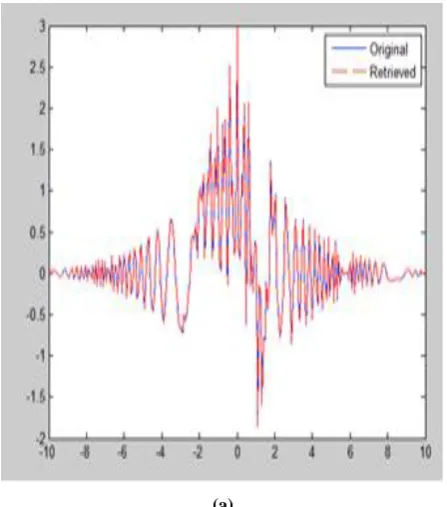
Filtering results for the signal in time-frequency domain are found using MATLAB R2011a. The MSE of the retrieved signal is calculated with the original signal. The results show that the filtering done in fractional domain gives better concentration as well as resolution. The time-bandwidth product of the signal concentration in fractional domain is also calculated which verifies that the concentration is better in the fractional domain. The spectrograms shown in figure 5 (a),(b) are for STFT and STFrFT respectively. Figure 6(a),(b) show the original and retrieved signals for STFT and STFrFT respectively.

(a)

(b)

Fig.5: (a) Spectrogram of filtering with STFT for a chirp signal. (b) Spectrogram of filtering with STFrFT in

fractional Fourier domain for the same chirp.

(a)

(b)

Fig.6: (a) original and retrieved signal after STFT filtering. (b) original and retrieved signal after STFrFT

filtering.

Table I: MSE Comparison for STFT and STFrFT Filtering.

STFT STFrFT

0.0953 0.000931

The Mean Square Error (MSE) comparison shows a wide range of improvement in the received signal for STFrFT filtering.

STFrFT can be used for a wide range of applications where chirp signals are involved.

5.

CONCLUSION AND FUTURE

SCOPE:

We can conclude that the filtering of chirp signals done in fractional Fourier domain is better than that done in the Fourier domain. The analysis also shows reduced mean square error which is an indication of the better signal retrieval method. The transform is also helpful in eliminating the cross terms present in other TFDs. STFrFT filtering can be best used when the signals are replicas of SONAR or RADAR signals. For further enhancing the properties an optimized transform for Short time Fractional Fourier Transform can be used with an adaptive window size.

6.

ACKNOWLEDGEMENTS:

We would express our gratitude towards all the faculty members who have always been helpful and supportive. We would also love to thank Mr. Ankit Rana who has always rendered his support towards us, our loving family and caring friends for keeping our morale high and for their confidence in us.

7.

REFERENCES

[1] C. Capus and K. Brown, “Short-time fractional Fourier methods for the time-frequency representation of chirp signals,” J. Acoust. Soc. Amer.,vol. 113, no. 6, pp. 3253– 3263, Jun. 2003.

[2] L.Cohen. Time-frequency analysis [J]. IEEE Signal

[3] J.B.Wu, J.Chen, P.Zhong. Time frequency-based blind source separation technique for elimination of cross-terms in Wigner distribution [J]. Electronics Letters, vol.39, pp:475-477, May 2003.

[4] L. B. Almeida, “The fractional Fourier transform and time-frequency representations,” IEEE Trans. Signal Process., vol. 42, no. 11, pp. 3084–3091, Nov. 1994. [5] X. G. Xia, “On bandlimited signals with fractional Fourier

transform,” IEEE Signal Process. Lett., vol. 3, pp. 72–74, Mar. 1996.

[6] R. Tao, B. Deng, W. Q. Zhang, and Y. Wang, “Sampling and sampling rate conversion of band limited signals in the fractional Fourier transform domain,” IEEE Trans. Signal Process., vol. 56, no. 1, pp.158–171, Jan. 2008. [7] Ran Tao, Yan –Lei Li and Yue Wang, “Short Time

Fractional Fourier Transform and its Applications”, IEEE Trans. Signal Process., vol. 58, no. 05,pp 2568-2580, May 2010.