Comparison of Propagation Model Accuracy for Long
Term Evolution (LTE) Cellular Network
Sami A. Mawjoud
Electrical Engineering Department University of Mosul
Mosul, Iraq
ABSTRACT
This paper investigates three different empirical propagation models for the next 4th generation known Long Term Evolution (LTE) in the (2-3) GHz band in urban and suburban areas. The suitability of these models are compared with actual field measurement at 2.6 GHz in Erbil city-Iraq. Tuning method is suggested to fit the experimental results of path loss with the propagation models.
Keywords
Long Term Evolution (LTE), Path Loss Models, Propagation Measurement, Model Tuning.
1. INTRODUCTION
Long Term Evolution (LTE) is the 4th generation cellular system. The followings are the main objectives of LTE [1]:
Increased downlink speed of 100 Mbps and uplink speed of almost 50 Mbps.
The channel will have a scalable bandwidth from 1.3 MHz to 20 MHz.
Supporting both Frequency Division Duplex (FDD) and Time Division Duplex (TDD).
All IP Network (Flat Network Architecture). A standard based interface that can support
multitude of users types.
All new wireless systems undergo careful planning [2][3] process, where coverage, capacity and cost-efficiency issues are investigated and optimized. Coverage is an essential part of wireless system design and it is used to verify whether or not the system under design is capable of meeting the given coverage requirements. There are two propagation model techniques:
Theoretical analysis method based on radio propagation.
Actual measurement and statistical method based on large amount of test data and empirical formula.
The radial tracking model integrated into the planning software which can be put into commercial use, such as Volcano model and Winprop model, and they are representations of propagation model research through the theoretical analysis method, but this type of model requires a high precision (at least 5m), including 3D digital map of building information. Accuracy of model predication is closely related to the precision and accuracy to digital map.
In the actual and statistical method for propagation model, the most famous statistical model is Okumura model. This model is propagation model represented by curves and was built by okumura based on a large amount of test data collected in Japan. On basis of okumura model, the regression method is
used to fit out resolution empirical formula to facilitate computation.
The selection of suitable radio propagation model for LTE is of great importance. The choice of the empirical model accompanied by actual field measurement in the intended area is of vital importance. Therefore path loss measurement and prediction in different areas environment (urban, suburban, etc…) is necessary. Finally, adaption of tuning method is suggested for the theoretical model to fit the experimental results.
2. PATH LOSS MODELS
Propagation lo ss (LP) is the different value between the radiated power (PT) and the received power (PR).
d … )
2.1 Okumura-Hata Model
Okumura-Hata model [4] uses empirical data to determine the path loss (LP) in dB given by equation (2).
LP(urban) (dB) = 69.55+26.16 log10 (fc) -13.82 log10 (hb) – a (hm) + (44.9-6.55 log10 (hb)) log10 (d) …. (2)
Where fc: is the frequency in MHz
hb: is the BTS effective transmitter antenna height in meter.
hm: is the effective mobile receiver antenna height in meter.
d: is the distance between Base Station (Bs) and the Mobile Station (Ms) in Kilometers.
a(hm): is the correction factor for effective Ms antenna height which is a function of the size of the coverage area. where the correction factor a(hm) for suburban and rural area is
a(hm) = (1.1 log10 (fc)- 0.7) hm – (1.56 log10 (fc)- 0.8) … 3)
For Urban area the correction factor a(hm) is
a(hm) = 823 (log10 (1.54 hm)) 2
– 1.1 for fc< 300MHz … 4)
a(hm) = 3.2 (log10 (11.75 hm))2 – 4.97 for fc> 300MHz … 5) The path loss for Suburban area is:
LP(Suburban)(dB) = LP(urban) – 2 log10(fc/28)2 -5.4 …. 6)
And the path loss for open area is:
LP(Open)(dB) = LP(urban) – 4.78 log10 (fc) 2
+18.33 log10 (fc) -40.94 …. 7) The limitations of Okumura-Hata model are:
42
2.2 Cost-231 Okumura-Hata Model
An extension of Okumura-Hata model is the cost-231 Hata model [5][6]. The model extends the frequency range up to 2000 MHz.
Lp(cost-321) (dB) = 46.3+33.9 log10 (fc) -13.82 log10 (hb) – a (hm) + (44.9-6.55 log10 (hb)) log10 (d)+ Cm …. 8)
For large city (urban area) the correction factor a(hm) is given by Eq. (5). While a(hm) for suburban or rural areas is given by Eq. (3).
Cm=0 for median sized cities and suburban areas. Cm = 3dB for metropolitan areas
2.3 SUI Model
Stanford University Intern (SUI) model [7] is developed for IEEE 802.16 Broadband wireless access working group. It is suited for frequencies above 1900MHz. The main difference from other models is that the path loss exponent is treated as a random variable in addition to the shadowing effects. The basic path loss ( PL) of this model along with its correction factors is given as:
PL (dB) = A+ 10ϒ log10 (d/do) + Xf + Xh + S … 0)
Where : PL is the path loss in dB
A is the free space path loss given as:
A= 20log10 (4do/) … )
Where do is the reference distance 100 meters from the Bs
ϒ = a- bhb + c/hb ….. 2)
Where: hb is the height of base station and (a,b,c) represent the terrain for which the values are selected as shown in table (1).
Xf is the correction factor for frequency given as
Xf = 6 log10 (f/2000) …. 3)
Xh is the correction factor for Bs height given as
Xh = -10.8 log10 (hr/2000) …. 4)
hr is the height of Ms receiver antenna and f in MHz.
Xh in Eq. (14) is used for terrain type A and B. For terrain C the below expression is used.
Xh = -20 log10 (hr/2000) …. 5)
Table (1) SUI model numerical values for different terrain categories.
Mode Parameters
Terrain A (hilly/moderate
to heavy tree density)
Terrain B (hilly/light tree
density of flat / moderate to
heavy tree density)
Terrain C (flat/light
tree density)
a 4.6 4.0 3.6
b(m-1) 0.0076 0.0065 0.005
c 12.6 17.1 20
2.3 Log-Distance Propagation Model
The power law path loss model [8][9] is one of the simplest path loss model to be used it consists of two propagation environment related parameters and two reference parameter which are used to adjust the model to the corresponding propagation environment. The path loss PL(d) is used to predict the mean path loss values and is given below.
PL(d) (dB) = PL(do) + 10 n log10 (d/do) …. 6)
PL(do) is the reference path loss at reference distance (do) in dB.
n is a variable represent the propagation exponent fading variation over the mean path loss value. The reference path loss value is approximated either using free space path loss formula or through field measurements at distance do. The propagation environment related parameter n and the center frequency, the propagation environment and the antenna height are given.
The propagation exponent n is typically used to classify propagation environment and it describes how quickly the signal level attenuates as a function of distance.
3. PROPAGATION MODEL TUNING
The purpose of propagation model tuning is to minimize the error between the predicted path loss values and the measurements [9][10].
3.1 Cost-231 Hata Model Tuning
Linear Least Squares Method (LLSM) can be used to achieve a minimum mean error and acceptable standard deviation (Std) between measure and predict path loss [11][12]. The mathematical analysis of LLSM is shown as below[13][14].
First, defined the parameters of all equations used below which are:
LP is the theoretical path loss from Hata Model. Lm is measured path loss. L is the difference between predicted and measured path loss. A1 is additional factor for constant attenuation. A2 is additional factor for attenuation about distance (d). Ltuned is the tuned Hata propagation model after modification for each terrain environment.
Eq. (8) can be written as :
LP (dB) = K1 +33.9 log10 (f) -13.82 log10 (hb) –a(hm) +K2 log10(d) +(-6.55 log10 (hb) log10 (d)) + Cm
By adding A1 and A2 factors for tuning purpose, the Ltuned equation can be written as:
Ltuned (dB) = (K1+A1) +33.9 log10 (f) -13.82 log10 (hb) –a(hm) +(K2 + A2) log10(d) +(-6.55 log10 (hb) log10 (d)) + Cm … 7)
Reasoning for only K1 and K2 is that for each test of a certain station f, hb, hm are all fixed values but the distance is variable [9].
L= (LP – Lm)
The error equation can be written as :
, 2) i- 2l 0di 2 n
i … 8)
(20) By using LLSM to find the values of A1 and A2 to obtain a lower value of E(A1,A2).
0 and
2 0 … 9)
By solving Eq.(19) the result is:
)
n
i
l 0di n
i
2 i n
i
.. 2
From Eq.(20) and Eq. (21) result a matix equation :
n
i n
i
)
n
i
n
i
il 0di n
i
i n
i
22)
3.2 SUI Propagation Model Tuning
The mathematical analysis of SUI tuning using Carmer’s method is shown below.
Eq. (10) can be written as:
PL (dB) = C + n B + S … 23)
Where: S is the correction factor, B=10 log10 (d/do), do=100m, C= A+ Xf + Xh.
, i mi
2 n
i
… 24)
0 and 0 … 25)
Eq. (24) can be s lved usin Carmer’s determinant based method.
n Bi + S= Lmi – C …. 26)
n
n
m – C mn – C
27)
3.2 Log-Distance Propagation Model
Tuning
The mathematical analysis of log-distance tuning model using Carmer’s method is shown below. Eq. (16) can be written as:
PL (dB) = A+ n B … 28)
Where: A is free space path loss given in Eq. (11), B=10 log10 (d/do), do=100m.
n i mi
2 n
i
… 29)
n Bi = Lmi – A ...(30)
n n
m – mn –
… 3 )
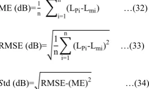
The verification statistical parameters which used in this paper are Mean Error (ME), Root Mean Square Error (RMSE) and Standard deviation (Std)[2][10].
d ) n i- mi) n
i … 32)
d )
n i mi) 2 n
i
… 33)
td d ) - )2 … 34)
4. MEASUREMENTS PROSCEDURE
The aim of radio measurement is to measure the signal strength transmitted from a test transmitter by a receiver at different distance within coverage area. The radio measurement data files are used to optimize the parameters in the path loss prediction model to achieve optimal predicted signal level compared to measured signal level. The measurements procedure included the following:
Define models required to recreate coverage of different physical environments: such as a Cost-321 Hata, SUI, Log-distance models which are chosen for tuning process in this paper.
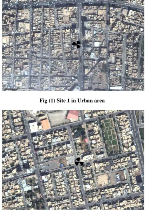
Site selection survey to find suitable sites for each environment: the location of test site have been selected carefully in order to cover each dominant clutter types Urban and Suburban in Erbil city as shown in fig(1) and(2).
Tx and Rx equipment: Table (2) show the parameters of two Bss, the received equipment is a Test Mobile System Measurement Unit which is known (TEMS Investigation) as a data collection software tool is used. TEMS is designed for signal strength measurement and a lap-top computer it was used to control TEMS unit (USB Modem) andto store the measured data with Global position System (GPS) having external antenna.
Assessment and preparation of data collection:
Before the collected data can be used , appropriate filtering was performed to verify its validity and remove erroneous data. A distance filtering has been applied minimum distance 50m and maximum distance 2km. an additional signal strength filtering has been performed to collected data, the signal range applied is (-40 to -120)dBm.
Table(2) Base Station Parameters
Bs2_ suburban Bs1_ urban
Bs Name
18dB 18dB
Antenna Gain
28.3m 35m
Antenna Height
7o 6o
Antenna Downtilt
2600MHz 2600MHz
Frequency Band
20MHz 20MHz
Channel Bandwidth
46.2 dBm 46.2 dBm
Max Tx Power
-115 dBm -115 dBm
[image:3.595.317.466.144.233.2]44
Fig (1) Site 1 in Urban area
Fig (2) Site 2 in Suburban area
5. RESULTS AND DISCUSSION
To verify the proposed mathematical models for different propagation models tuning, a comparison between predicted path loss and measured path loss data have been carried out for LTE site (operating at 2.6GHz) for urban and suburban environments in Erbil city.
For verification and comparison between the tuned propagation models in order to find the close fitting model to measure data. Statistical parameters mean error, root mean square error and standard deviation have been considered.
Fig (3) and Fig (4) show comparison between the measured data and predicted path loss for Cost-231 Hata, SUI and Log-distance models as a function of Log-distance. It can be observed from fig(3) and fig(4) that the optimum model which is close to the measured path loss is the tuned Cost-231 Hata model which have lowest mean error (ME) reaching zero as compared to other propagation models. Tables (3,4,6) represent the results of the statistical tuning process for each model.
The tuned SUI model also have good performance with mean error 0.32dB, the tuned log-distance model have the lowest performance as compared to other models but it is still acceptable from the practical view of tuning process because the mean error is lower than 1dB. From tables (3,4,6) it can be concluded that the mathematical models which used are suitable for tuned propagation models because all tuned model (SUI, Cost-231 Hata, Log-distance) have lower mean error and acceptable standard deviation, as in table(5) which represent the value of parameters before tuning and table (6).
Fig(3) Comparison of the optimized Path loss with measured data for urban area site.
Fig(4) Comparison of the optimized Path loss with measured data for suburban area site.
Table (3) Log-Distance Propagation Model Parameters.
RMSE [dB] Mean
Std. [dB] Mean Error [dB] Pathloss
Exponent (n) Clutter Class
8.5 8.3
-0.68 4.8
Urban Area
7.82 7.81
0.43- 3.6
Suburban Area
Table (4) SUI Propagation Model Parameters After Tuning Process
RMSE [dB] Mean Std. [dB] Mean Error [dB] Correction Factor(S) [dB] Pathloss Exponent (n) Clutter Class
8.82 8.83
0.32 -68
6.38 Urban
Area
8.28 8.3
12.0 -65
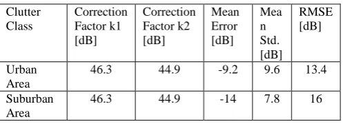
[image:4.595.51.284.72.410.2] [image:4.595.305.534.74.256.2] [image:4.595.306.532.299.488.2] [image:4.595.310.544.540.602.2]Table (5) Cost231-Hata Propagation Model Parameters Before Tuning Process.
RMSE [dB] Mea n Std. [dB] Mean Error [dB] Correction Factor k2 [dB] Correction Factor k1 [dB] Clutter
Class
13.4 9.6
-9.2 44.9
46.3 Urban
Area
16 7.8 -14 44.9
46.3 Suburban
Area
Table (6) Cost231-Hata Propagation Model Parameters After Tuning Process.
RMSE [dB] Mean Std. [dB] Mean
Error [dB] Correction Factor k2 [dB] Correction Factor k1 [dB] Clutter
Class
7.85 7.8
0 73.9
49.82 Urban
Area
7.6 7.63 -0.0037 72.2
43.8 Suburban
Area
6. CONCLUSION
In this paper a proposed optimization method of path loss models using least square method is presented. The models tuning have be excuted to fit empirical path loss models to actual field measurements. Analytical and measured results concluded that the performance of tuned Cost-231 Hata model is the best among other considered models. The mean error of the cost-231 Hata model for urban area is reduced to zero, the mean standard deviation value is reduced to 7.8dB and the root mean square error reduced to 7.85dB. Hence the Cost-231 Hata model is recommended to be used for propagation prediction in Erbil city.
7. REFERENCES
[1] LTE an Introduction, White paper, Ericsson AB, 2009.
[2] L. Kalzar, J. Prokopec, "Propagation Path Loss Models For Mobile Communication", IEEE International Conference Radioelektronika, 2011.
[3] M. Didarul and M. Razaul, " Comparison Study of Path Loss Models of WiMAX at 2.5 GHz Frequency Band", International Journal of Future Communication and Networking, Vol. 6, No. 2, April 2013.
[4] Hata M., "Empirical Formula For Propagation Loss in Land Mobile Radio Services", IEEE Transaction on Vechicular Technology Vol. 29, No. 3, 1980.
[5] Goldsmith A., " Wireless Communication", USA, Cambridge University Press, 2005.
[6] A. Yawardhana, V. Wassel, J. Closby, D. Sellars, M. Brown, " Comparison of Empirical Propagation Path Loss Models For Fixed Wireless Access Systems", Proceeding of the 61 IEEE Vehicular technology conference, 2005.
[7] N. Shabbit, M. Saidq, H. Kashif, and R.Ullah, " Comparison of Radio Propagation Models For Long Term Evolution (LTE) Network", International Journal of Next generation networks, Vol. 3, No. 3, September 2011.
[8] M. Lanovic, S. Rimac, and K. Bejuk, " Comparison of Propagation Models Accuracy for WiMAX on 3.5 GHz, IEEE International Conference on Electronics, 2007.
[9] J. Demertriow, R. Mackenzi. " Propagation Basics", September 30, 1998, pp. 39-42. Available online on www.scribd.com/doc/7218261/Propagation-Basics.
[10] B. Yesin, I. Hakki, " Mobile Radio Propagation Measurements and Tuning the Path Loss Model in urban Area at GSM-900 Band Istanbul-Turkey", Fall 60th Vehicular Technology conference, No. 6, Los Angeles CA, 2004.
[11] M. Yang, W. Shi, " A linear Least Square Method for Propagation Model Tuning for 3G Radio Network Planning", Fourth International Conference on neutral Computation, IEE Computer Society, Vol. 5, pp. 150-154, 2008.
[12] K. Diawuo, T. Cemberbatch, " Data Fitting to Propagation Model Using Least Square Algorithm: A Case Study in Ghana", International Journal of Engineering Science, Vol. 2, No. 6, June 2013.
[13] B. Castro, M. Pinheiro, G. Canalcante, " Comparison Between Known propagation Models Using Least Square Tuning Algorithm on 5.8 GHz in Amazon Region Cities", Journal of Microwaves, Optoelectronics Application, Vol. 10, No. 1, June 2011.
[14] Simi I., Santi I., and Zermi B.," Minimax LS Algorthim for Automatic Propagation Model Tuning" Proceeding of the 9th Telecommunications Forum (TELFOR 2001), Belgrade, Nov 2001.
[image:5.595.44.293.100.190.2]