Development of Elastic Modulus Density Chart for a Typical Femur Bone Model

©IJRASET 2015: All Rights are Reserved

352

Development of Elastic Modulus - Density Chart

for a Typical Femur Bone Model

Gabriel Oladeji Bolarinwa1, Nishant Kumar Singh2, Sanjay Kumar Rai3

1,2

Research Fellow, 3Assistant Professor, School of Biomedical Engineering IIT (BHU), Varanasi, India.

Abstract-Finite element (FE) analysis has been widely used to study the behaviour of bone or implants in many clinical applications. One of the main factors in analyses is the realistic behaviour of the bone model, because the behaviour of the bone is strongly dependent on a realistic bone material property assignment [1]. The determination of inhomogeneous material properties of bone in finite element analysis is currently based on two converting formula that convert the computed tomography number, Hounsefield Units and Grayvalues into bone density and then into Young’s modulus. However, there are variations between studies and no standardized set of formulae exists [2].The objective of this study is to develop Elastic Modulus- Density chart for a typical femur bone using one of the existing mathematical model for material properties assignment. This mathematical model was applied to the femur obtained from a CT scan and MIMICS software and imported to ANSYS 15.0.The density and Young’s modulus of the bone were generated. The result obtained was used to develop a chart that can be used for experimental purposes. The future work will be carried out on the validity of this chart.

Keywords: Density, Elastic modulus, Femur, Orthotropic, Material Assignment

I. INTRODUCTION

Bone material presents a complex behaviour involving heterogeneous and anisotropic mechanical properties. Moreover, bone is a living tissue, therefore its microstructure and mechanical properties evolve with time, in a process called bone remodelling. This phenomenon has been studied from a long time, and there are many numerical models that have been formulated in this sense to predict the density distribution in various bones, mainly in the femur. [3]

The finite element (FE) method has been increasingly adopted in the past few years to study the mechanical behaviour of biological structures, whereas computed tomography (CT) has been widely used in FE modeling of bone. It is well known that CT images can provide fairly accurate quantitative information on bone geometry and it can be also related with the mechanical properties of bone tissues. Based on CT data, the assignment of bone material properties to FE meshes is a fundamental step in the model generation. The appropriate bone material properties are mainly based on the relationships between CT numbers, gray values, Hounsfield Units (HU), and bone mechanical properties. In fact, there are different experimental relationships available in the literature relating the HU with the density and other mechanical characteristics of the bone tissue. [4] An emerging focus on the investigation and analysis of the biomechanics of human bone is to generate preclinical information which is helpful for the researcher and orthopedicians has been seen. For this, a geometric model that acts like a natural bone has increasingly been considered to better understand the mechanics of the bone. Mechanical properties of bone are inhomogeneous which differentiate the bone geometrical structure as cortical and cancellous bone, in the same way as man-made engineering materials Nishant Kumar Singh, Richa Braru, et al described the processes involved in transforming the CT scan into solid model using SimpleWare Scan IP software. In this work, the same procedural steps were followed but MIMICS software was used in place of SimpleWare Scan IP. The transformation and segmentation processes will not be stressed in this work. The objective of this study was to develop a chart from existing orthotropic material mathematical models, that is, a close to realistic material property assignment critical for finite Element (FE) analyses of typical bone specimens.

II. MATERIALS AND METHOD/ METHODOLOGY

Collection of raw data that represent the desired anatomy of the bone, (CT scan or MRI of natural femoral joint). Generation of the solid model of the femur using MIMICS software.

©IJRASET 2015: All Rights are Reserved

353

Importing the model materials into ANSYS and generate result for material properties. Use the generated results to develop the desired chart.

III. MATERIAL ASSIGNMENT

Bone is an inhomogeneous structure consisting of two types of material; cortical and cancellous bone. Both types of bone tissue are orthotropic materials with specific structures and specific mechanical behaviours. The relationship between CT numbers and the effective density of bone tissue is well known from the literature. Most authors have used the mechanical properties needed for a finite element model predicted from CT numbers. For a realistic assignment of bone material properties it is necessary to know nine independent elastic constants and the spatial orientation of the principal axes of orthotropy. While elastic constants have been described in detail for both types of bone tissue (cortical and cancellous); however material property assignment with regard to the principal axes of orthotropy remains a problem. Also, the structure and orientation of cortical and cancellous bone has been described in a number of papers. The general problem lies in implementing the orientation of the material into the FE model as an orthotropic material. While it is not difficult to assign the principal axes of orthotropy to cortical bone structure, the opposite is true in the case of Trabecular/cancellous bone [5]. The structure of cancellous bone is highly variable throughout its volume, and therefore a clear definition of the principal axes of orthotropy is impossible.

A. Mathematical Models Applied For Materials Assignment

According to Wolff’s Law, there is a remarkable similarity between the trabecular architecture of proximal femur and the stress trajectories. In this research work, the femur model was divided into 10 segments from the proximal end through the cortical are to the distal ends. The proximal and the distal ends are similar in properties because they are the spongy parts (Cortical/trabecular) of the femur bone. Based on the gray values (GV) and the threshold values in Hounsfield (HU) the mathematical relationships below were applied in MIMICS (Fig.1-3) to calculate the density (ρ) across the segments and the Modulus of elasticity (E) in all the

directions.

= 0.0000464 + 1 (g/cm3) ………. 1; where is the effective density.

The bone materials are dependent on effective density. The bone materials properties are as a function of effective density are described below:

EC= 2065ρ3.09 ……….……… 2

ET= 1904ρ1.64 ……….……… 3

υc= υT = 0.3 ………... 4

E = Young Modulus, υ is the Poisson ratio, C and T represent cortical and trabecular (cancellous) bone. The functions for an orthotropic definition of the bone properties are: ECx = ECY= 2314ρ1.57 ……… 5

ECz = EC= 2065ρ3.09 ……… 6

ETx = ETY= 1157ρ1.78 ……… 7

ETz= 1904ρ1.64 ……… 8

Gxy = Gxymaxρ2 / ρmax2 ………. 9

Gyz = Gyzmaxρ2 / ρmax2 ……… 10

Gzx = Gzxmaxρ2 / ρmax2……… 11

Where G is the shear modulus (Mpa), ρmax is the maximum density. Gxymax, Gyzmax and Gzxmaxare 5.71Mpa, 7.11MPa and 6.58MPa respectively.

©IJRASET 2015: All Rights are Reserved

354

Figure 1: Histogram showing the material distribution on femur model

©IJRASET 2015: All Rights are Reserved

355

Figure: 3. Material assignment on the femur model

IV. RESULTS

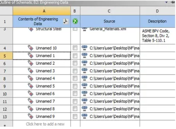
The femur with assigned materials was then imported into ANSYS 15.0. The necessary tools and commands were employed (figure 2 after which the ten (10) material properties were generated as displayed in (figure 4) and recorded in table 1 below.

©IJRASET 2015: All Rights are Reserved

356

0 1 2 3 4 5 6 7 8 9 10 11 12 13 14 15

Y o u n g M o d u lu s (E +9 x P a

Number of Segments

Young Modulus across the bone

segments

Young Modulus

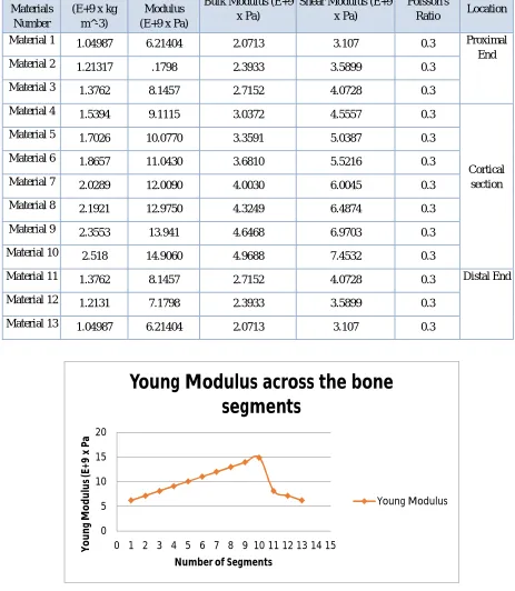
Table 1: Bone Materials and their Orthotropic Properties

Figure 5: Modulus of Elasticity across the bone segments Materials

Number

Density (E+9 x kg

m^-3)

Young's Modulus (E+9 x Pa)

Bulk Modulus (E+9 x Pa)

Shear Modulus (E+9 x Pa)

Poisson's

Ratio Location

Material 1 _{1.04987 6.21404 2.0713 3.107 0.3} Proximal End Material 2 _{1.21317 .1798 2.3933 3.5899 0.3}

Material 3 _{1.3762 8.1457 2.7152 4.0728 0.3}

Material 4 _{1.5394 9.1115 3.0372 4.5557 0.3}

Cortical section Material 5 _{1.7026 10.0770 3.3591 5.0387 0.3}

Material 6 _{1.8657 11.0430 3.6810 5.5216 0.3}

Material 7 _{2.0289 12.0090 4.0030 6.0045 0.3}

Material 8 _{2.1921 12.9750 4.3249 6.4874 0.3}

Material 9 _{2.3553 13.941 4.6468 6.9703 0.3}

Material 10 _{2.518 14.9060 4.9688 7.4532 0.3}

Material 11 _{1.3762 8.1457 2.7152 4.0728 0.3} Distal End

Material 12 _{1.2131 7.1798 2.3933 3.5899 0.3}

©IJRASET 2015: All Rights are Reserved

357

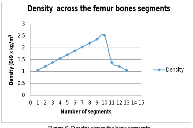
0 1 2 3 4 5 6 7 8 9 10 11 12 13 14 15

D e n si ty ( E+ 9 x k g/ m 3

Number of segments

Density across the femur bones segments

Density

Figure 6: Density across the bone segments.

V. DISCUSSION

Figures 5&6 were generated from table 1 .These figures show the profile of the mechanical properties across the segments of the bone. The density and the stresses followed the pattern of the material arrangement. At the proximal (head to neck), the cortical and the distal (condyles) ends, the material arrangement were calculated according to the gray values and this is the factor that determines the bone densities.

Figure 7: Modulus of Elasticity against density

The proximal and the distal ends have approximately the same properties because they are both spongy in nature. This was also confirmed in figures 1& 3. The histogram shows the material distribution across the whole part of the bone and also looking at the colours in figure 3, the colour distribution in condyles and the femur/femoral neck are almost the same. This indicates that they have similar properties. Figure 7 was obtained by plotting the values of the densities and the modulus obtained in from table 1.

y = 5.919x R² = 1

0 1 2 3 4 5 6 7 8 9 10 11 12 13 14 15 16

0 0.5 1 1.5 2 2.5 3

M

o

d

u

lu

s

o

f

El

a

st

ic

it

y

(E

+9

x

P

a

)

Density (E+9 x kg/m

Elastic Modulus versus Density

©IJRASET 2015: All Rights are Reserved

358

VI. CONCLUSION

Material property goes a long way in obtaining a better FE analysis of human bone for better results. There is a need to develop a realistic mechanical property chart for different types of bones. This can serve as a chart relating the elastic modulus and density for a typical femur bone and could be used for experimental purposes though the validity has not been ascertained. Due to wide diversity in the anthropometric measurements of the femur population and varying biological structures, this chart must be evaluated carefully before use.

REFERENCES

[1] Vaclav Baca , Zdenek Horak ,Petr Mikulenka et al , Comparison of an inhomogeneous orthotropic and isotropic material models used for FE analyses. Elsevier

Journal of Medical Engineering and Physics volume 30 (2008) pp 924–930.

[2] Weng-Pin Chen, Jui-Ting Hsu et al, Determination of Young’s Modulus Of Cortical Bone Directly from Computed Tomography: A Rabbit Model, Journal of

the Chinese Institute of Engineers, Vol. 26, No. 6, pp. 737-745 (2003) 737

[3] M. A. P´erez, P. Fornells, J. M, Validation of Bone Remodelling Models Applied to different bone Types using MIMICS

[4] Nishant Kumar Singh, Richa Braru, et al, Development and Validation Of Robust 3D -Solid Model of Human Femur using CT Data, International Journal of

Advances in Science Engineering and Technology, ISSN: 2321-9009 Volume- 2, Issue-3, July-2014

[5] Brinckmann, P, Frobin, W., Hierholzer, E., (1981). Stress on the articular surface of the hip joint in healthy adults and persons with idiopathic osteo-arthrosis of

the hip joint. J Biomech, 14, (149-156), ISSN 0044-3220.

[6] A.E Yousif, M.Y Aziz, Biomechanical analysis of human femur during normal working and standing up IOSR Journal of Engineering, Volume 2, Issue 8 ,

2012 pp 13-19.

[7] Brinckmann, P, Frobin, W., Hierholzer, E., (1981). Stress on the articular surface of the hip joint in healthy adults and persons with idiopathic osteo-arthrosis of