5
IX
September 2017
Optimization of Co
2
Laser Beam Cutting Process
Parameters for Machining Of AISI 9255 Spring
Steel
Renangi Sandeep 1, S Bala Anki Reddy 2, S Jaya Kishore 3
1, 2
Assistant Professor, Department of Mechanical Engineering, Siddartha Institute of Science and Technology, Puttur, A.P., India – 517583
3
Assistant Professor, Department of Mechanical Engineering, SVCE, Tirupathi, A.P., India – 517501
Abstract: The present work deals with the process parameters optimization of continuous wave CO2 laser cutting of AISI 9255
spring steel. In the present study four process variables such as laser power, cutting speed, laser pressure and focal distance are
considered and experimentation are carried out based on L27 orthogonal array (OA). The cut quality responses such as surface
roughness and kerf taper are measured for every experimental run. To optimize process parameters TOPSIS method is employed. The aim of optimization is to minimize surface roughness and kerf taper characteristics.
Keywords: CO2 Laser beam cutting, spring steel, Kerf taper, TOPSIS, L27 OA
I. INTRODUCTION
The laser was developed in 1960s due to its precision and high intensity has been widely used in the field of fine cutting of sheet metals. Lasers remain well known and a very flexible mechanism for producing various micro-structures in this modern era, particularly in upgrading of engineering materials. Laser Beam Machining (LBM) is one of the innovative non-conventional machining process that actuality contemporarily used for shaping virtually entire range of engineering materials wherever complex shapes in request precise, fast and force-free processing. In addition, marking, drilling, and welding applications, cutting is the most irregularly useful LBM process.
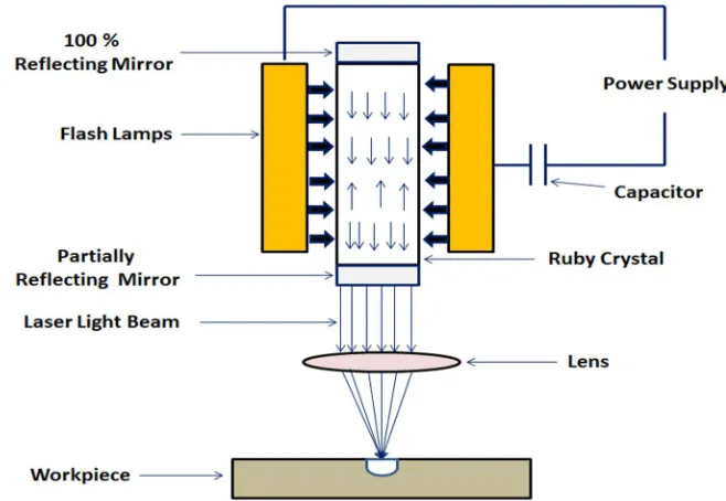
[image:2.612.138.467.489.716.2]Laser beam cutting is a non-contact type; thermal energy based unconventional machining process in which an excessive intensity laser beam is concentrated at a spot and material gets melted or evaporated at that spot. The molten metal was removed from the melting pool by supplying the high pressure co-axial assisted gas as show in Fig. 1. The efficiency of the laser cutting process be influenced by mechanical properties of the material to be cut and then also based on the thermal and some extent optical properties.
There are many researchers have been studied laser beam cutting process. Some of literatures are B S Yilbas [1] has studied the Striation formation due to the slow drifts and disturbances in various parameters during the laser cutting process. The effects of laser power, cutting speed and energy coupling factor on the kerf size are investigated. His work has shown that increasing laser power and energy coupling factor increase the kerf width size. Also, small changes in laser power, cutting speed and energy coupling factor modify the kerf width to a great extent. Dayana Espinal and Aravinda Kar [2] have developed A simple mathematical model to relate kerf depth to laser power, laser scanning speed and kerf width during laser cutting. Asano et al. [3] have shown that the range of processing conditions which allow cutting is determined by the energy input per unit area. The values of roughness of the cutting surface on both entry and exit sides of the plates can be reduced if the cutting speed is 1000 mm/min or higher. They change
little at small values if the heat input per unit area is within a range under 20 J/mm2. Cutting with small heat input always results in
better finish of cut surface. Uslan.I [4] has investigated the influence of laser power and cutting speed variations on the kerf width size. A lump parameter analysis is introduced when predicting the kerf width size and an experiment is conducted to measure the kerf size and its variation during the cutting process. He has found that the workpiece surface influences significantly the kerf width size. He has also shown that the variation in the power intensity results in considerable variation in the kerf size during the cutting, which is more pronounced at lower intensities. Zhang et al [5] have proposed a synthetic evaluation method for laser cutting quality. B S Yilbas et al [6] using a CO2 laser with variable pulse frequency and Oxygen, as assisting gas, at different pressures have investigated the cutting process. SEM and X ray diffraction are carried out to obtain micrographs and oxide compounds formed in the dross. They have found that the liquid layer thickness increases with increasing laser output power and reduces with increasing assisting gas velocity. The mechanics of dross formation has been studied by using the relation between kinetic energy of the melt film and the local temperature. Striation produced during the laser cutting affects the surface roughness, appearances and geometry of laser cut products. Lin Li, M. Sobih and P.L. Crouse [7] have given a theoretical model to predict the critical cutting speed at which striation-free cutting takes place. It is also observed that at cutting speeds above the critical cutting speed, striation reappears and surface roughness increases with the cutting speed.
In this present paper, two output responses are taken such as kerf taper and surface roughness have been optimized simultaneously during continues wave co2 laser beam cutting of AISI 9255 spring steel using approach of Topsis method. The control factors taken as laser power, gas pressure, focal distance and cutting speed. The plate material of AISI 9255 spring steel having thickness of 8 mm is taken into consideration. Firstly, Experiments have been performed on AISI 9255 spring steel work piece based upon Taguchi experimental design L27 orthogonal array. The results obtained from Taguchi-based experiment have been used in Topsis for finding optimal solutions.
II. EXPERIMENTATION
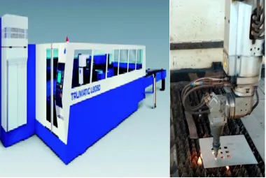
The experiments are conducted on High power CO2 Laser Machining centre model no Trumatic L6050, made by GSI group laser division, United Kingdom which is available with M/s. Meera Laser Solutions (I) PVT. LTD. Chennai, Tamilnadu. The maximum average power produced at laser is 3200W. In this research profile cutting of AISI 9255 spring steel is carried out at by varying the input parameters. The chemical composition of the material is given in Table I.
Table I: Chemical Composition Of Aisi 9255 Spring Steel
% C Cr Si Mn P V S Fe
Min 0.45 0.80 0 0.50 0 0 0
Balance
max 0.55 1.20 0.50 0.80 0.06 0.15 0.06
A. Experimental setup
significant effect on cut edge quality such as surface roughness and taper kerf. In the present work, surface roughness and taper kerf are considered as the decision variables and trial samples of square profile cutting with the dimensions of 10 x 10 mm are performed by varying one of the process variables to determine the working range of each process variable.
Fig 2: The CO2 laser-machining center (Trumatic L6050) Fig. 3: CO2 Laser Machining process
Table II: Experimental Conditions
Factors Units Levels
I II III
Power KW 1.6 1.8 2.0
Cutting Speed mm/sec 4000 4250 4500
Gas Pressure Bar 2.0 2.5 3.0
Focal Distance mm 1 1.1 1.2
B. Design of Experiments
Design of experiments (DOE) is used to find out the effect of different process response parameters on different control factors and for getting the relation between them. For giving the minimum no of experimental runs, we will get the required amount of information it will save the machine time and cost of the experiment. In taguchi method the experiments are performed as per the standard orthogonal arrays (OA). The selection of orthogonal array depends on the total degree of freedom (DOF). In the present investigation to check the DOFs in the experimental design for the three-level test, the four main factors take 8 (4 × (3-1)) DOFs. For three second order interactions (A×B, A×C, B×C) is 16 (4 × (3-1) × (3-1)) and the total DOFs required is 24 (8+16). Here the L27 OA (DOF: 26) has been selected. The design of experiments is given in Table III to run the experiments.
III. EXPERIMENTAL RESULTS AND DISCUSSIONS
[image:4.612.119.499.118.373.2]A. Topsis method
TOPSIS stands for technique for order preference by similarity to ideal solution. This method was developed by Hwang and Yoon in the year 1995. Technique for order preference by similarity to ideal solution (TOPSIS) is based on the idea that the chosen alternative should have the shortest distance from the positive ideal solution and on the other side the farthest distance of the negative ideal solution. The ideal solution is a hypothetical solution for which all attribute values correspond to the minimum attribute values in the data base. TOPSIS thus gives a solution that is not only closest to the hypothetically best but also farthest from the hypothetically worst. The steps followed for the TOPSIS in the present research work are given below.
1) Step 1: Decision matrix is normalized by using the following equation:
rij =
∑ --- Equ. (1)
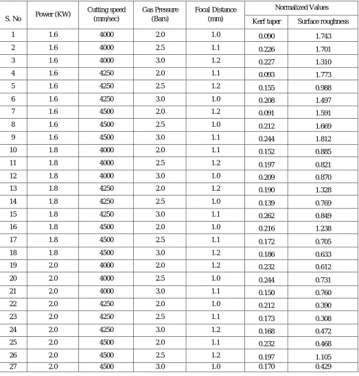
where i = 1 ⋯ m and j = 1 ⋯ n. aij represents the actual value of the ith value of jth experimental run and rij represents the corresponding normalized value. The normalized values of kerf taper and surface roughness are presented in Table IV.
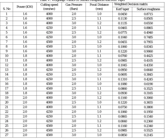
2) Step 2: Weight for each response is calculated. Here, equal weightage is given to all the responses. Therefore, wj = 0.50.
The weights for all the responses are given in Table V.
Vij = Wi × rij --- Equ. (2)
where i = 1 ⋯ m and j = 1 ⋯ n. wj represents the weight of the jth attribute or criteria.
S. No Power (KW)
Cutting speed (mm/sec) Gas Pressure (Bars) Focal Distance (mm) Kerf tapper (degree) Surface roughness (μm)
1 1.6 4000 2.0 1.0 0.303 5.851
2 1.6 4000 2.5 1.1 0.758 5.710
3 1.6 4000 3.0 1.2 0.761 4.398
4 1.6 4250 2.0 1.1 0.311 5.951
5 1.6 4250 2.5 1.2 0.521 3.317
6 1.6 4250 3.0 1.0 0.697 5.024
7 1.6 4500 2.0 1.2 0.306 5.340
8 1.6 4500 2.5 1.0 0.711 5.602
9 1.6 4500 3.0 1.1 0.820 6.083
10 1.8 4000 2.0 1.1 0.511 2.970
11 1.8 4000 2.5 1.2 0.660 2.756
12 1.8 4000 3.0 1.0 0.702 2.920
13 1.8 4250 2.0 1.2 0.6365 4.457
14 1.8 4250 2.5 1.0 0.465 2.582
15 1.8 4250 3.0 1.1 0.881 2.849
16 1.8 4500 2.0 1.0 0.725 4.156
17 1.8 4500 2.5 1.1 0.577 2.368
18 1.8 4500 3.0 1.2 0.625 2.125
19 2.0 4000 2.0 1.2 0.780 2.055
20 2.0 4000 2.5 1.0 0.819 2.455
21 2.0 4000 3.0 1.1 0.502 2.551
22 2.0 4250 2.0 1.0 0.711 1.309
23 2.0 4250 2.5 1.1 0.582 1.034
24 2.0 4250 3.0 1.2 0.565 1.584
25 2.0 4500 2.0 1.1 0.779 1.570
26 2.0 4500 2.5 1.2 0.661 3.709
3) Step 3: In this step, the worst alternative (twj) and the best alternative (tbj) are determined from the weighted normalized values (tij). These values are used to determine the separation measures. Table VI shows the Best and worst values of output parameters.
Table IV: Normalized Values Of Surface Roughness And Kerf Taper
S. No Power (KW)
Cutting speed (mm/sec)
Gas Pressure (Bars)
Focal Distance (mm)
Normalized Values
Kerf taper Surface roughness
1 1.6 4000 2.0 1.0 0.090 1.743
2 1.6 4000 2.5 1.1 0.226 1.701
3 1.6 4000 3.0 1.2 0.227 1.310
4 1.6 4250 2.0 1.1 0.093 1.773
5 1.6 4250 2.5 1.2 0.155 0.988
6 1.6 4250 3.0 1.0 0.208 1.497
7 1.6 4500 2.0 1.2 0.091 1.591
8 1.6 4500 2.5 1.0 0.212 1.669
9 1.6 4500 3.0 1.1 0.244 1.812
10 1.8 4000 2.0 1.1 0.152 0.885
11 1.8 4000 2.5 1.2 0.197 0.821
12 1.8 4000 3.0 1.0 0.209 0.870
13 1.8 4250 2.0 1.2 0.190 1.328
14 1.8 4250 2.5 1.0 0.139 0.769
15 1.8 4250 3.0 1.1 0.262 0.849
16 1.8 4500 2.0 1.0 0.216 1.238
17 1.8 4500 2.5 1.1 0.172 0.705
18 1.8 4500 3.0 1.2 0.186 0.633
19 2.0 4000 2.0 1.2 0.232 0.612
20 2.0 4000 2.5 1.0 0.244 0.731
21 2.0 4000 3.0 1.1 0.150 0.760
22 2.0 4250 2.0 1.0 0.212 0.390
23 2.0 4250 2.5 1.1 0.173 0.308
24 2.0 4250 3.0 1.2 0.168 0.472
25 2.0 4500 2.0 1.1 0.232 0.468
26 2.0 4500 2.5 1.2 0.197 1.105
Table V: Weightage Values Of Surface Roughness And Kerf Taper
S. No Power (KW)
Cutting speed (mm/sec)
Gas Pressure (Bars)
Focal Distance (mm)
Weighted Decision matrix
Kerf taper Surface roughness
1 1.6 4000 2.0 1.0 0.0450 0.8715
2 1.6 4000 2.5 1.1 0.1130 0.8505
3 1.6 4000 3.0 1.2 0.1135 0.6550
4 1.6 4250 2.0 1.1 0.0465 0.8865
5 1.6 4250 2.5 1.2 0.0775 0.4940
6 1.6 4250 3.0 1.0 0.1040 0.7485
7 1.6 4500 2.0 1.2 0.0455 0.7955
8 1.6 4500 2.5 1.0 0.1060 0.8345
9 1.6 4500 3.0 1.1 0.1220 0.9060
10 1.8 4000 2.0 1.1 0.0760 0.4425
11 1.8 4000 2.5 1.2 0.0985 0.4105
12 1.8 4000 3.0 1.0 0.1045 0.4350
13 1.8 4250 2.0 1.2 0.0950 0.6640
14 1.8 4250 2.5 1.0 0.0695 0.3845
15 1.8 4250 3.0 1.1 0.1310 0.4245
16 1.8 4500 2.0 1.0 0.1080 0.6190
17 1.8 4500 2.5 1.1 0.0860 0.3525
18 1.8 4500 3.0 1.2 0.0930 0.3165
19 2.0 4000 2.0 1.2 0.1160 0.3060
20 2.0 4000 2.5 1.0 0.1220 0.3655
21 2.0 4000 3.0 1.1 0.0750 0.3800
22 2.0 4250 2.0 1.0 0.1060 0.1950
23 2.0 4250 2.5 1.1 0.0865 0.1540
24 2.0 4250 3.0 1.2 0.0840 0.2360
25 2.0 4500 2.0 1.1 0.1160 0.2340
26 2.0 4500 2.5 1.2 0.0985 0.5525
27 2.0 4500 3.0 1.0 0.0850 0.2145
Table VI Best And Worst Values Of Output Parameters
Output parameter vbj vwj
Kerf Taper 0.045 0.131
Surface roughness 0.154 0.906
4) Step 4: The separation of each alternative from positive ideal solution (PIS) and negative ideal solution (NIS) is calculated as
= ∑ − --- Equ. (3)
= ∑ − --- Equ. (4)
TABLE VII SEPERATION MEASURE VALUES
S. No Power (KW)
Cutting speed (mm/sec)
Gas Pressure (Bars)
Focal Distance (mm)
Separation measures
S S
1 1.6 4000 2.0 1.0 0.718 0.093
2 1.6 4000 2.5 1.1 0.700 0.058
3 1.6 4000 3.0 1.2 0.506 0.252
4 1.6 4250 2.0 1.1 0.733 0.087
5 1.6 4250 2.5 1.2 0.342 0.415
6 1.6 4250 3.0 1.0 0.597 0.160
7 1.6 4500 2.0 1.2 0.642 0.140
8 1.6 4500 2.5 1.0 0.683 0.076
9 1.6 4500 3.0 1.1 0.756 0.009
10 1.8 4000 2.0 1.1 0.290 0.467
11 1.8 4000 2.5 1.2 0.262 0.497
12 1.8 4000 3.0 1.0 0.287 0.472
13 1.8 4250 2.0 1.2 0.512 0.245
14 1.8 4250 2.5 1.0 0.232 0.525
15 1.8 4250 3.0 1.1 0.284 0.482
16 1.8 4500 2.0 1.0 0.469 0.288
17 1.8 4500 2.5 1.1 0.203 0.555
18 1.8 4500 3.0 1.2 0.169 0.591
19 2.0 4000 2.0 1.2 0.168 0.600
20 2.0 4000 2.5 1.0 0.225 0.541
21 2.0 4000 3.0 1.1 0.228 0.529
22 2.0 4250 2.0 1.0 0.073 0.711
23 2.0 4250 2.5 1.1 0.042 0.753
24 2.0 4250 3.0 1.2 0.091 0.672
25 2.0 4500 2.0 1.1 0.107 0.672
26 2.0 4500 2.5 1.2 0.402 0.355
27 2.0 4500 3.0 1.0 0.073 0.693
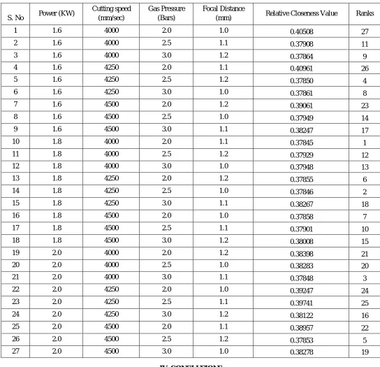
5) Step 5. The closeness coefficient of each alternative (CCi) is calculated as
= --- Equ. (5)
Table Viii Relational Closness Values And Their Ranks
S. No Power (KW)
Cutting speed (mm/sec)
Gas Pressure (Bars)
Focal Distance
(mm) Relative Closeness Value Ranks
1 1.6 4000 2.0 1.0 0.40508 27
2 1.6 4000 2.5 1.1 0.37908 11
3 1.6 4000 3.0 1.2 0.37864 9
4 1.6 4250 2.0 1.1 0.40961 26
5 1.6 4250 2.5 1.2 0.37850 4
6 1.6 4250 3.0 1.0 0.37861 8
7 1.6 4500 2.0 1.2 0.39061 23
8 1.6 4500 2.5 1.0 0.37949 14
9 1.6 4500 3.0 1.1 0.38247 17
10 1.8 4000 2.0 1.1 0.37845 1
11 1.8 4000 2.5 1.2 0.37929 12
12 1.8 4000 3.0 1.0 0.37948 13
13 1.8 4250 2.0 1.2 0.37855 6
14 1.8 4250 2.5 1.0 0.37846 2
15 1.8 4250 3.0 1.1 0.38267 18
16 1.8 4500 2.0 1.0 0.37858 7
17 1.8 4500 2.5 1.1 0.37901 10
18 1.8 4500 3.0 1.2 0.38008 15
19 2.0 4000 2.0 1.2 0.38398 21
20 2.0 4000 2.5 1.0 0.38283 20
21 2.0 4000 3.0 1.1 0.37848 3
22 2.0 4250 2.0 1.0 0.39247 24
23 2.0 4250 2.5 1.1 0.39741 25
24 2.0 4250 3.0 1.2 0.38122 16
25 2.0 4500 2.0 1.1 0.38957 22
26 2.0 4500 2.5 1.2 0.37853 5
27 2.0 4500 3.0 1.0 0.38278 19
IV.CONCLUSIONS
The scope of present paper was the optimization of process parameters in laser beam machining of AISI 9255 spring steel using TOPSIS Method. The process parameters examined in this investigation are cutting speed, laser power, gas pressure and focal distance. The following conclusions are made.
A. The optimized process parameter setting is laser power 1.8 KW, cutting speed of 4000 mm/sec, gas pressure of 2.0 bars and 1.1
mm focal distance.
C. The proposed experimental and statistical approach is simple, useful, and a reliable methodology to optimize laser welding parameters efficiently. In future, this method can be used to optimize and improve other process parameters. Also, this method can be extended to study other machining processes.
REFERENCES
[1] B.S.Yilbas A., F.M.Arif, B.J.Abdul Aleem,, “Dross formation during laser cutting process”, J. Phys. D: Appl. Phys. 39,1451-1461 [2006]
[2] Dayana Espinal and Aravinda Kar (2000) , “Thermochemical modeling of oxygen assisted laser cutting”, Journal of Laser Applications, February, Volume 12,
Issue 1, pp 16 – 22
[3] Asano,Hiroshi, Suzuki,Jippei,Kawakami,Eguchi(2003), “Selection of parameters on laser cutting mild steel plates taking account of some manufacturing
purposes”, Fourth International symposium on laser precision microfabrication. Proceedings of SPIE, Volume 5063, pp 418-425.
[4] Uslan.I (2005), “CO2 laser cutting: kerf width variation during cutting”, Proceedings of the I MECH E Part B Journal of Engineering Manufacture, Number B8,
August 2005, pp. 571-578(8).
[5] Lawrence Yao, Hongquiang Chen and Wenwu Zhang (2004), “Time scale effects in laser material removal”, International Journal of Advanced Manufacturing
Technology
[6] B.S.YilbasA., F.M.Arif, B.J.Abdul Aleem, “Laser welding of low carbon steel and thermal stress analysis”, Optics & Laser Technology, Volume 42, Issue 5,
July 2010, Pages 760-768
[7] Lin Li, M. Sobih and P.L. Crouse (2007), “Striation free Laser Cutting of Mild Steel”, Sheets, CIRP Annals of Manufacturing Technology, Volume 56, Issue 1,