Optimal Side Lobes Reduction of Linear Array
Antenna Using Crow Search Algorithm
Jaspreet Kaur1, Dr. Sonia Goyal2
1
Student, Department of Electronics and Communication, Punjabi University, Patiala, Punjab
2
Asst. Prof., Department of Electronics and Communication, Punjabi University, Patiala, Punjab
Abstract: The aim of this paper is to introduce the novel metaheuristic crow search Optimization algorithm (CSA) to the electromagnetic and antenna community. Crow search algorithm is a population based method, mimicking the intelligent behavior of crows to proceed to a global solution. In this paper, CSA has been employed for the pattern optimization of linear antenna array by elements amplitude only and position only synthesis. Different designs examples are presented that illustrate the effectiveness of CSA for linear array optimization; so as to obtain an array pattern with minimum side lobe level (SLL) along with null placement in the specified directions. The results of CSA are validated by benchmarking them with the results obtained by ant lion optimization (ALO), particle swarm optimization (PSO) and grey wolf optimization (GWO) etc. Here, peak SLL and deep nulls obtained from crow search algorithm are improved up to -38 dB and -105 dB, respectively. These Simulation results suggest that using CSA may lead to finding promising results compared to the other algorithms in terms of solution accuracy, easy to implement and convergence rate.
Keywords: linear antenna array, side lobe level (SLL), Null Depth, First null beam width, Crow Search Algorithm.
I. INTRODUCTION
The antenna is a fundamental part or back bone of the wireless communication which is utilized in short and long distance communications. The IEEE standard definition in terms for antennas defines the antenna as "a means for radiating or receiving radio waves". All the fast increasing use of wireless communications needs an enhancement in characteristics of the network such as capacity, quality of service and coverage [1]. A single antenna can't meet these requirements, because of its limited performance in terms of gain and directivity. Alternatively, the use of this antenna in an array makes it more efficient to achieve the optimum solutions. In additional words, an antenna array comprises multiple fixed point antennas arranged in such a manner that its effective radiation pattern is interfere constructively in desired direction and cancelled in opposite direction to achieve a desired radiation pattern [2]. Each of these antenna elements, while functioning has their own induction field. Therefore, the vector addition of all the individual elements radiated fields provides total field of array. An extensive study about the literature reported that, Pattern synthesis of antenna array can be expressed by controlling the parameters which depend on the structure of the antenna. Among these parameters, we can refer to the geometric configuration of array, element spacing, excitation amplitude, excitation phase and the pattern of each element [3].
In literature, several metaheuristic/evolutionary algorithms have been showing their promising performance for solving most real-world optimization problems that are extremely nonlinear. All metaheuristic algorithms use a certain tradeoff of randomization and local search to reach to a global solution [4]. For this reason, the scope of metaheuristic has expanded tremendously in the last two decades. Some optimization algorithms which have been successfully applied to the synthesis of array pattern: are genetic algorithm (GA) based on natural selection [2], Grey wolf optimization [4], Cat swarm optimization [7], Ant lion algorithm based on hunting behavior of ant lions [8], gravitational force optimization based on Newtonian law of gravity [9], Cuckoo search algorithm [14], particle swarm optimization (PSO) based on social behavior of bird flocking [16] etc.
In this paper, a newly developed nature inspired algorithm, Crow Search Algorithm (CSA) is employed for first time to the linear array pattern optimization. In the present work, two types of optimization are demonstrated to achieve a directional radiation pattern with low side lobe levels around the main beam. First type is the excitation current amplitudes optimization and the second one is
elements position optimization by taking φ = 0. The main goal is to reduce side lobes with the constraint of beam width and to
sophisticated ways and hide and retrieve food across seasons. Based on these properties, CSA attempts to simulate the intelligent behavior of the crows to find the solution of optimization problems.
The rest of this paper is organized as follows. In section II, the synthesis of linear antenna array geometry, calculation of the array factor and fitness function are explained and section III, deals with the concepts of the Crow search algorithm (CSA). The synthesized patterns with low SLL for different array elements are presented in section IV. Finally, in section V conclusions are drawn.
II. FORMULATION OF THE DESIGN PROBLAM
Linear array is one of the most commonly used array structure to achieve desired radiation characteristics. The problem considered here is to minimize the side lobe level and null placement by optimizing the antenna array parameters such as amplitude, phase and distance of the individual array elements. In our study, Consider the geometry of a simplest linear antenna array with N elements placed in straight line as shown in Fig 1. It is assumed that the antenna elements are symmetric with regard to the centre of linear array, and these elements create the variety of patterns when packed as an array [1].
Fig.1. Symmetric N linear antenna array geometry [2]
The array factor of an antenna array is defined as the product of element factor and spacing factor and it is independent of the antenna type. The calculation of such array factor for any antenna array geometry has a great importance to determine its radiation characteristics and many other electromagnetic properties. Array factor for symmetric array with 2N geometry in azimuth plane can be calculated as (1)
E(θ) = 2.∑ A cos[k. x . cos(θ) +φ ] (1)
Where N denotes the number of array elements, k is wave number, θ denotes azimuth angle. A , φ and x denotes the excitation
amplitude, phase and location of nth array element respectively. If we assume that all elements have uniform amplitude and phase
excitations (that is A =0 and φ = 0). Therefore, array factor equation again simplified as (2)
E(θ) = 2.∑ A cos[k. x . cos(θ)] (2)
The normalized form of the equation (1) is given as in dB in equation (3)
E(θ) dB = 20∗log ( )
( ) (3)
Where, max E(θ) is the maximum value of array factor E(θ) and it is obtained for θ= π 2.
III. A CROW SEARCH OPTIMIZATION
is search space and the global solution of the problem is relating to the best food source of the environment. In view of these similarities, CSA attempts to simulate the intelligent behavior of the crows to discover the solution of optimization issues. To approve the effectiveness of CSA simulations have been executed on different mathematical benchmark functions and on some
real-world engineering design problems [3].
It is expected that there is a d-dimensional environment including various crows. The quantity of crows (flock size) is N and the
position of crow i at time iter in the search space is determined by a vector x, (i = 1, 2, … . , N; iter = 1, 2, … . . iter ) where
x, = x, x, … x,
and iter is the maximum number of iterations. Each crow has a memory in which the position
of its hiding place is memorized. At iteration iter, the position of hiding place of crow i is shown by m, . This is the best position
that crow i has gotten up until now. For sure, in memory of each crow the position of its best experience has been retained. Crows
move in the environment and scan for better substances sources (concealing spots).
It is expected that at iteration iter, crow j needs to visit its covering place m, . At the same iteration, crow i takes after crow j to
deal with the hiding place of crow j. In this situation, two states may happen:
State 1: Crow j does not realize that crow i is tailing it. Accordingly, crow i will approach to manage the hiding place of crow j. For
this circumstance, the new position of crow i is gotten as:
x, = x, + r × fl, × (m, − x, )
(4)
Where, r is an arbitrary (random) number with uniform distribution in the vicinity of 0 and 1.
State 2: Crow j understands that crow i is tailing it. Therefore, with a particular ultimate goal to protect its food from being
appropriated, crow j will fool crow i by taking off to another position of the hunt space. Absolutely, states 1 and 2 can be determined
as:
x, = x, + r × fl, × (m, − x, ) r ≥ AP,
a random position otherwise (5)
Where, r is a subjective number with uniform distribution in the region of 0 and 1 and refers the AP, awareness probability of
crow j at iteration iter [3].
(a) state 1 (fl < 1) (b) state 2 (fl > 1)
Fig. 2 Flowchart of state 1 and state 2 [3]
IV. CSA IMPLEMENTATION FOR OPTIMIZATION
Pseudo code of CSA is shown in Fig. 2. The step-wise procedure for the implementation of CSA is given in this section.
A. Initialize problem and adjustable parameters. The optimization problem, decision variables and constraints are defined. Then,
the adjustable parameters of CSA (flock size (N), maximum number of iterations ( ), flight length ( ) and awareness
probability (AP)) are valued.
B. Initialize position and memory of crows N crows are randomly positioned in a d-dimensional search space as the members of
Crows = ⎣ ⎢ ⎢ ⎢ ⎡ … … . . . . . . . . . . . . … ⎦⎥ ⎥ ⎥ ⎤ (6)
The memory of each crow is initialized. Since at the initial iteration, the crows have no experiences, it is assumed that they have hidden their foods at their initial positions.
Memory = ⎣ ⎢ ⎢ ⎢ ⎡ … … . . . . . . . . . . . . … ⎦⎥ ⎥ ⎥ ⎤ (7)
C. Evaluate fitness (objective) function For each crow, the quality of its position is computed by inserting the decision variable
values into the objective function.
D. Generate new position
E. Check the feasibility of new positions The feasibility of the new position of each crow is checked. If the new position of a crow
is feasible, the crow updates its position. Otherwise, the crow stays in the current position and does not move to the generated new position.
F. Evaluate fitness function of new positions The fitness function value for the new position of each crow is computed.
Update memory
G. It is seen that if the fitness function value of the new position of a crow is better than the fitness function value of the
memorized position, the crow updates its memory by the new position.
H. Check termination criterion Steps 4–7 are repeated until is reached. When the termination criterion is met, the best
position of the memory in terms of the objective function value is reported as the solution of the optimization problem [3].
Fig. 3 Flowchart of CSA
V. EXPERIMENT RESULTS
This section presents the simulated results of linear antenna array optimization by using the CSA optimization algorithm. The CSA is applied to linear antenna array in order to determine the optimized antenna element current amplitudes to minimize the peak SLL and to place nulls in the desired directions based on the MATLAB platform. Design examples A, B and C are used to describe the optimization results. In design example A, the optimized current excitation amplitudes are illustrated to minimize the peak SLL and place deep nulls in the specified region. Design example B illustrates the application of CSA to determine the optimized antenna element positions in order to minimize maximum SSL in antenna array radiation pattern. The convergence of novel approach CSA is characterised in part C. There are fewer parameters which are adjusted before start optimization by CSA. The maximum iterations
used for each run are set to be 1000, population size (N) is 20, awareness probability (AP) is 0.2 and the flight length (fl) is 2.5.
A. Element excitation amplitude optimization: In this section, the various linear array design steps are used for minimization of SLL for amplitude control to be in the range (0, 1). The synthesis of linear array is initialized with inter-element distance
d=0.56 which is same as uniform array, and constant phase angle as = 0. The fitness function presented for maximum SSL
suppression is illustrated as follows (8):
= min 20∗ 10( ) (8)
Where, AF is the normalized array factor and it is synthesized using CSA. The experiment is performed for N = 10, 16 and 20 elements for amplitude only control in order to achieve desired radiation pattern. In step 1 the optimized current excitation amplitudes for 2N = 10 are illustrated in TABLE 1, by taking uniform element distance. A graphical comparison of the optimized linear array factor, in the case of amplitude only control pattern synthesis is shown in Fig 4. It is seen from Fig 4. that the proposed algorithm CSA provides a better reduction in SLL as compared to arrays optimized using other optimization algorithms such as ALO [8], BBO, GWO [4] and PSO [16]. All simulation results have been plotted as the array factor (AF) versus azimuth angle plot. The following table shows the optimized current excitation amplitude of elements of the linear array, used in our simulations.
TABLE 1 optimized current amplitudes of the 10 element linear array
Method Excitation current amplitudes
ALO 1.0000 0.8959 0.6957 0.4935 0.2966
PSO 1.0000 0.9010 0.7255 0.5120 0.4088
GWO 1.0000 0.8962 0.6963 0.4935 0.2964
BBO 1.0000 0.8526 0.6586 0.4601 0.5101
CSA 0.9976 0.9106 0.7403 0.5017 0.3514
The excitation amplitude is greater at the centre of array and decreases towards array edges. From fig, it is concluded that CSA
provides maximum peak SLL reduction in the regions [0o, 70o] and [110o, 180o], as compared to other evolutionary optimizations
[image:6.612.74.538.264.347.2]approaches. The proposed algorithm CSA gives a peak SLL of -37.32 dB. The peak SLL has been lowered from -26.1 dB to -37.32 dB (by dB) as compared to ALO [8] optimization array, from -24.90 dB to -37.32 dB (by dB) as compared to PSO [16], from -31.43 dB to -37.32 dB (by dB) as compared to BBO [17] and from -29.8 dB to -37.32 dB (by dB) as compared to GWO [4] optimization array.
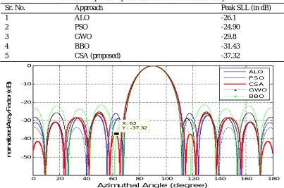
TABLE 2 Optimized peak SLL for 10 element linear array
Sr. No. Approach Peak SLL (in dB)
1 ALO -26.1
2 PSO -24.90
3 GWO -29.8
4 BBO -31.43
5 CSA (proposed) -37.32
Fig. 4 Array radiation pattern for 10 element linear array
0 20 40 60 80 100 120 140 160 180
-50 -40 -30 -20 -10 0
X: 63 Y: -37.32
Azimuthal Angle (degree)
n
o
rm
a
li
z
e
d
A
rr
a
y
F
a
c
to
r
(d
B
)
ALO PSO CSA GWO
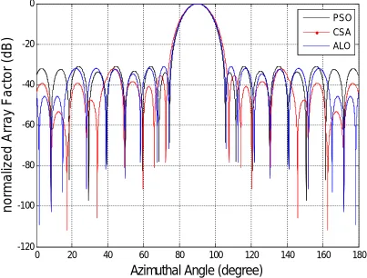
[image:6.612.104.507.448.715.2]The design example B describes the synthesis of 16 element linear antenna array for control the excitation current amplitudes with the constraint of null placement in specified region. The corresponding comparison normalized radiation pattern for an element array of 16 is depicted in Fig 5.
[image:7.612.99.515.478.568.2]Fig. 5 array radiation pattern for 16 element linear array
TABLE 3 Optimized peak SLL for 16 element linear array
Method Optimized current amplitudes
PSO 1.0000 0.9521 0.8605 0.7372 0.5940 0.4465 0.3079 0.2724
ALO 1.0000 0.9344 0.8521 0.7044 0.6000 0.4000 0.3003 0.2002
CSA 0.9778 0.9202 0.8213 0.6743 0.5232 0.3801 0.2591 0.1845
The comparative results of optimized excitation current amplitudes for 16 element antenna array are illustrated in TABLE 3. The current values obtained by proposed CSA optimization approach have been compared with that of ALO and PSO. Further the obtained peak SLL reduction results are given in TABLE 4.
TABLE 4 comparative analysis of peak SLL and null depth by PSO, ALO and CSA algorithms Method
PSO ALO CSA
Null depth (dB) -78.22 -78.45 -91.78
Peak SLL (dB) -33.9 -31.6 -35.71
It is seen from Table 4 that the peak SLL reduction have been given by CSA (-35.71 dB) is better than PSO (by – 1.81 dB) and ALO (by – 4.11 dB). Also, it is observed from fig 6 that minimum null depth is -91.78 dB in desired direction.
0 20 40 60 80 100 120 140 160 180
-120 -100 -80 -60 -40 -20 0
Azimuthal Angle (degree)
n
o
rm
a
liz
e
d
A
rr
a
y
F
a
c
to
r
(d
B
)
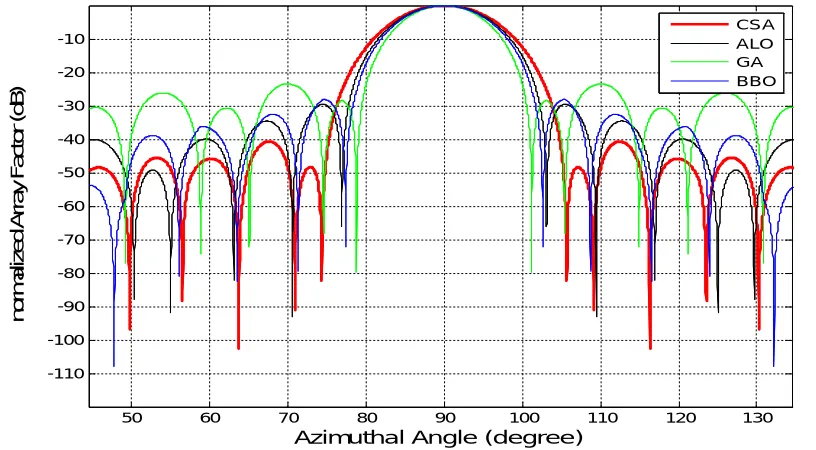
[image:7.612.113.499.635.697.2]Fig. 6 array radiation pattern for 20 element linear array
TABLE 5 Optimized peak SLL for 20 element linear array
Method Optimized current amplitudes
ALO 1.0000 0.9790 0.9188 0.8135 0.7005 0.6000 0.4649 0.3301 0.2155 0.1114
GA 0.9427 0.8175 0.8034 0.6692 0.6665 0.5830 0.4538 0.4317 0.3763 0.3395
BBO 1.0000 0.9747 0.9264 0.8575 0.7022 0.6242 0.4799 0.3607 0.2369 0.1234
CSA 0.9089 0.8680 0.7934 0.6817 0.5641 0.4352 0.3227 0.2158 0.1273 0.0779
TABLE 6 Optimized peak SLL for 20 element linear array
Method ALO GA BBO CSA
Peak SLL (dB) -29.61 -30.35 -28.14 -46.27
In TABLE 6, it is seen that, the minimum SLL obtained by CSA is -46.27 dB. There is an improvement in low side lobe level by using CSA then ALO by -16.66 dB, GA by -15.92 dB and BBO by -18.23 dB.
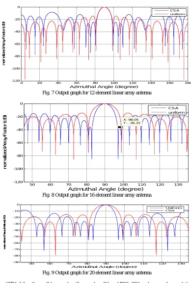
B. Element position optimization: To illustrate the effectiveness of proposed approach CSA, the no of elements 12, 16 and 20 are
considered along with antenna positions (x ) optimization. Further, the excitation amplitude (I ) and phase (φ ) are assumed as
constant for position only synthesis. The crow search algorithm (CSA) with fitness function shown in figure is used for
determining the optimized element positions (x ). The comparative array pattern for CSA and uniform array is shown in Fig 7.
TABLE 7 comparative output of peak SLL and FNBW using CSA and uniform array No. of elements
N
Uniform array CSA
SLL (dB) FNBW (deg) SLL (dB) FNBW (deg)
12 -14.49 20.3 -24.35 12.2
16 -14.51 18.9 -36.25 13.8
20 -15.64 19.6 -31.24 14.1
50 60 70 80 90 100 110 120 130
-110 -100 -90 -80 -70 -60 -50 -40 -30 -20 -10
Azimuthal Angle (degree)
n
o
rm
a
liz
e
d
A
rr
a
y
F
a
c
to
r
(d
B
)
Fig. 7 Output graph for 12 element linear array antenna
Fig. 8 Output graph for 16 element linear array antenna
Fig. 9 Output graph for 20 element linear array antenna
C. Convergence of FPA: Like other well known algorithms such as GA and PSO, CSA makes use of a population of crows to explore the search space. By use of a population the probability of finding a good solution and escaping from local minima increases. Parameter setting is one of the drawbacks of algorithms since it is time consuming work. Algorithms which have fewer parameters to adjust are easier to implement.
0 20 40 60 80 100 120 140 160 180
-120 -100 -80 -60 -40 -20 0
Azimuthal Angle (degree)
n o rm a liz e d A rr a y F a c to r (d B ) CSA uniform
50 60 70 80 90 100 110 120 130
-120 -100 -80 -60 -40 -20 0 X: 98.05 Y : -36.25
Azimuthal Angle (degree)
n o rm a liz e d A rr a y F a c to r (d B ) CSA uniform
50 60 70 80 90 100 110 120 130
-90 -80 -70 -60 -50 -40 -30 -20 -10 0
Azimuthal Angle (degree)
[image:9.612.117.499.106.275.2](a) (b)
[image:10.612.96.521.102.462.2](c)
Fig.10 convergence curves for Fitness (a) for N=12 (b) for N=16 (c) for N=20
In CSA, flight length and awareness probability are 2 parameters. Where, GA and PSO have 3 and 4 parameters respectively. A Figure 10 shows the convergence of the fitness function versus the no. of iterations. It is observed that although FPA is simpler to implement and also yields improved performance, but it takes more number of iterations to converge on to the optimum solutions as compared to PSO.
VI. CONCLUSION
In this paper, a systematic approach of crow search algorithm (CSA) technique is introduced and used for the optimization of uniform linear antenna array with non-uniform element positions. The main advantage of CSA over the other nature inspired evolutionary algorithms is that CSA have very few parameters to adjust such as awareness probability (AP) and flight length (fl) only, which in turn makes it very easier to implement. We apply the crow search algorithm (CSA) to optimize the excitation amplitudes as well as element positions of linear antenna array. Some numerical and simulated results of linear antenna array patterns are illustrated which shows that CSA provides maximum SLL reduction and null depth (as -38 dB and -105 dB respectively) as compared to PSO, BBO, GWO and ALO.
REFERENCES
[1] C.A. Balanis: Antenna Theory: Analysis and Design, John Wiley and Sons, Hoboken, NJ, USA, 2005.
[2] Adam Raniszewski, "Radiation pattern synthesis for RADAR application using Genetic Algorithm", 21st International Conference onMicrowave Radar and
Wireless Communications, 2016.
[3] A. Askarzadeh, “A novel metaheuristic method for solving constrained engineering optimization problems: crow search optimization,” Computers &
Structures, vol. 169, pp. 1-12, 2016.
0 100 200 300 400 500
0 0.2 0.4 0.6 0.8 1 1.2 1.4 1.6x 10
-4
iteration No.
F
it
n
e
s
s
0 50 100 150 200 250 300 350 400 450 500 0
0.5 1 1.5 2 2.5 3 3.5 4
F
it
n
e
s
s
Iteration No.
0 50 100 150 200 250 300 350 400 450 500 0
1 2 3 4 5 6
Iteration No.
F
it
n
e
s
[4] Ashwin Kothari. "Optimal pattern synthesis of linear antenna array using grey wolf optimization algorithm." International Journal of Antennas and Propagation (2016).
[5] El-Hadi and Christophe Dumond et.al. "A novel Modified Invasive Weeds Optimization for linear array antennas nulls control." 2015 4th International Conference on Electrical Engineering (ICEE). IEEE, 2015.
[6] D.D. Dajab and K. Ahmad. "Synthesis of a Linear Antenna Array for Maximum Side-lobe Level Reduction." International Journal of Computer
Applications 85. (2014).
[7] Debalina Ghosh et al. "Linear Antenna Array synthesis using cat swarm optimization", AEU-International Journal of Electronics and Communications 68, 2014.
[8] Saxena, Prerna, and Ashwin Kothari. "Ant Lion Optimization algorithm to control side lobe level and null depths in linear antenna arrays." AEU-International
Journal of Electronics and Communications 70, no. 9 (2016): 1339-1349.
[9] Maryam Hesari and Ataallah Ebrahimzadeh."Introducing Deeper Nulls and Reduction of Side-Lobe Level in Linear and Non-Uniform Planar Antenna Arrays
Using Gravitational Search Algorithm," Progress In Electromagnetics Research B, Vol. 73, 2017.
[10] Mahmoud, Korany Ragab. "Synthesis of unequally-spaced linear array using modified central force optimization algorithm." IET Microwaves, Antennas & Propagation 10, no. 10 (2016).
[11] Li, Xiangtao, and Minghao Yin. "Linear antenna array synthesis using orthogonal artificial bee colony algorithm." Journal of Computational and Theoretical
Nanoscience 10, (2013).
[12] Florine Enache and Andrei Enache, "Multi-Criteria Optimization of Non-Uniform Linear Antenna Array using Genetic Algorithms," IEEE 2016.
[13] Lei Chen and Xiao-Wei Shi, "An Iteration Method of Sidelobe Suppressing of Unequally Spaced Array," 3rd Asia-Pacific Conference on Antennas and Propagation, IEEE 2014.
[14] Shuang Liang and Geng Sun, "Sidelobe-level suppression for linear and circular antenna arrays via the cuckoo search–chicken swarm optimization algorithm,"
IET Microwaves, Antennas & Propagation 2016.
[15] V.S Gangwar and S P Singh, "Side Lobe Level Suppression in Randomly Spaced Linear Array Using Genetic Algorithm," IEEE International Microwave and
RF Conference, 2015.
[16] P.V.Florence, G.S.N Raju, “Synthesis of Linear Antenna Array using Accelerated Particle Optimization Algorithm,” International Journal of Computer
Applications (0975-8887) Volume 103- No.3, October 2014.
[17] Singh U., Kumar H., "Linear array synthesis using biogeography based optimization." Progress in electromagnetic research M 11, 25–36 (2010)
[18] Shaoqiu Xiao, Chunrong Zheng, Mei Li, “Varactor-Loaded Pattern Reconfigurable Array for Wide-Angle Scanning With Low Gain Fluctuation,” IEEE