Research on Saliency Detection

Research on Saliency Detection

Rainu R Padam

Computer Science Department

Viswajyothi College of Engineering and Technology, Mahatma Gandhi University

Abstract

—

computer vision viewpoint. The human pays unequal attention to what is seen in the world. When looking at some images, people are

usually attracted by some particular objects within the images. Other subjects appear uninteresting for them. This ability of withdraw from

some things in order to deal effectively with others is called attention. Detecting these areas of attention is called saliency detection.

Saliency detection has many applications, like object recognition, image segmentation, content-based retargeting, image retrieval, adaptive

image display,and advertising design. This survey presents five papers that describes various methods used for saliency detection. Some of

the selected papers uses multiple-instance learning technique for saliency detection. This survey also describes the avantages and

disadvantages of papers.

Keywords

—

I. INTRODUCTION

Saliency detection means detecting visually attracted regions. The visual system of human pays unequal attention to what is seen in the world. When looking at images in Fig. 1, people are usually attracted by flower, boat and dogs. Other subjects appear to be uninteresting for viewers. This ability of withdraw from some things in order to deal effectively with others is called attention.

The task of saliency detection is to extract the salient objects in an image, assuming that there is one or several salient ones within it. Salient object means visually attracted regions in images. The saliency value is generally denoted by a number scaled to [0, 1] and shown in a gray image. The greater value the pixel has, the higher possibility it is of being salient. There are many applications like object recognition, image segmentation, content-based retargeting , image retrieval, adaptive image display, and advertising design.

II. SALIENCY DETECTION BY MULTIPLE INSTANCE LEARNING

A. Image Segmentation

Each image is segmented using mean-shift algorithm to get bags. Mean Shift is a powerful and versatile non parametric iterative algorithm that can be used for lot of purposes like finding modes, clustering etc. Mean shift considers feature space as a empirical probability density function. If the input is a set of points then Mean shift considers them as sampled from the underlying probability density function. If dense regions are present in the feature space, then they correspond to the mode of the probability density function.

technique. For each data point, Mean shift defines a window around it and computes the mean of the data point. Then it shifts the center of the window to the mean and repeats the algorithm till it converges. After each iteration, consider that the window shifts to a more denser region of the dataset.

1) Kernel Density Estimation:Kernel density estimation is a non parametric way to estimate the density function of a random variable. This is usually called as the Parzen window technique. Kernel density estimation is a non parametric way to estimate the density function of a random variable. Kernel density estimator for a given set of d-dimensional points is

( ) = 1_ℎ ( −_ℎ )

where K(x) is kernel h, is bandwidth parameter (radius), n is the data point xi,i=1..n in d-dimension space Rd The estimate

of the density gradient is defined as the gradient of the kernel density estimateThe mean shift algorithm seeks a mode or local maximum of density of a given distribution.

2. Feature Extraction

The project utilizes low-, mid-, and high-level features. They are position, color,texture, scale, center prior, and boundary. Low level feature includes position, colour, texture and scale. Middile level feature extracted is center-prone prior. High level feature extracted is boundary.

1) Position: Connected pixels are prone to share similar saliency, whereas pixels far away tend to be differently salient. Therefore, the position of each instance is an essential factor for keeping the saliency consistent.

2) Color: This is the most frequently employed feature. However, for the choice of color spaces, there is not a noncontroversial agreement. HSV color space is used. With the most appropriate color space, color contrast is defined for each pixel, i.e.,

( , ) = ( , ) , ∊

where i is the examined pixel ( , )is the supporting region for defining the saliency of pixel i, and is the distance of color descriptors between i and j.

3) Texture: This is also a significant feature. The perceived textures can be described by different ways but are generally characterized by the outputs of a set of filters. The filter bank used is made of copies of a Gaussian derivative and its Hilbert transform, which model the symmetric receptive fields of simple cells in visual cortex. To be more specific, they are

( , ) = (1exp exp )

( , ) = ( ( , ))

where σ is the scale, l is the ratio of the filter, and C is a normalization constant. Similarly, texture contrast for each pixel is defined as

( , ) = ( , ) , ∊

where Ri and dt(i,j) have an analogous meaning with color

contrast.Since the texture descriptor is a continuous valued vector, the problem of computational complexity exists.

4) Scale: Scale is an effective property for identifying objects of different sizes. The difference between fine and coarse scales of color images is extracted to simulate the center-surround operations of visual receptive fields.

weighting principle will fail. Here a principle that emphasizes more on the close supporting region and less on the far one for the examined region is adopted.

6) Boundary: Boundary is different from what is traditionally known as edges. Edge is a low-level feature that indicates changes such as brightness, color, or texture. Boundary implies the ownership from one object to another. If there is a boundary in a region, it is more possible to indicate a salient object within this region.

3. Saliency Value Calculation

Saliency for each bag is calculated according to the learned model. A model is learned with the feature vectors by APR, Bag-SVM, and Inst-SVM, EM-DD.

1) Axis Parallel Rectangles: Axis parallel rectangle (APR) is constructed by starting with a single positive instance and growing the APR by expanding it to cover additional positive instances. It has three basic procedures.

 They are Grow: An algorithm for growing an APR with tight bounds along a specified set of features,

 Discrim: An algorithm for choosing a set of discriminating features by analyzing APR

 Expand: An algorithm for expanding the bounds of an APR to improve its generalization ability.

The algorithm works in two phases. In the first phase, the grow and discrim procedures are iteratively applied to simultaneously choose a set of discriminating features and construct an APR that has tight bounds along those features. In the second phase, the expand procedure is applied to expand these tight bounds. The backfitting algorithm is applied to construct a tight APR with bounds on all features. Then a subset of those features is selected as discriminating features.

2) Bag-SVM, and Inst-SVM: Two new formulations of multiple-instance learning is presented as a maximum margin problem. It tries to maximize the soft margin between two types of bags or instances. A linear discriminent is obtained.

There is atleast one instance from every positive bag in positive half space. All instances belonging to negative bags are in the negative half space. There are two approaches to modify and extend Support Vector Machines (SVMs) to deal with MIL problems. The first approach explicitly treats the pattern labels as unobserved integer variables, subjected to constraints defined by the (positive) bag labels. The second approach generalizes the notion of a margin to bags and aims at maximizing the bag margin directly.

3) EM-DD: A new multiple-instance learning technique that combines EM with diverse density algorithm is presented. EM-DD is a general purpose MI algorithm that can be applied with boolean or real value labels and make real value predictions. Here MI problem is converted to a single instance setting by using EM to esttimate the instance responsible for the label of the bag.

Fig. 1 Original image and its coresponding saliency maps

D. Advantages

 Consistent output

 Accurate saliency map

III. GLOBAL CONTRAST BASED SALIENT REGION DETECTION

A regional contrast based saliency extraction algorithm is proposed, which simultaneously evaluates global contrast differences and spatial coherence.

A contrast analysis is used for extracting high-resolution, fullfield saliency maps based on the following observations:

 A global contrast based method, which separates a large-scale object from its surroundings, is preferred over local contrast based methods producing high saliency values at or near object edges,

 Global considerations enable assignment of comparable saliency values to similar image regions, and can uniformly highlight entire objects,

 Saliency of a region depends mainly on its contrast to the nearby regions

 Saliency maps should be fast and easy to generate to allow processing of large image collections

A. Histogram Based Contrast

Histogram-based contrast (HC) method defines saliency values for image pixels using color statistics of the input image. The saliency of a pixel is defined using its color contrast to all other pixels in the image. The saliency value of each color is replaced by the weighted average of the saliency values of similar colors. The saliency value of a pixel Ik in

image I is defined as,

( ) = ( , ) ∊

where ( , )is the color distance metric between pixels and in the L*a*b*space. Rearranging such that the terms with the same color value cj are grouped together, saliency

value for each color is defined as,

( ) = ( , )

Where cl is the color value of pixel Ik n is the number of

different pixel colors, and fj is the frequency of pixel color cj

in image I.

B. Region Based Contrast

First segment the input image into regions, then compute color contrast at the region level, and define the saliency for

each region as the weighted sum of the region’s contrasts to

all other regions in the image. The weights are set according to the spatial distances with farther regions being assigned smaller weights.

Fig. 2 Original image and the coresponding saliency maps.

IV. LEARNING TO DETECT A SALIENT OBJECT

regionally, and globally. A Conditional Random Field is learned to effectively combine these features for salient object detection.

A. Multi-Scale Contrast

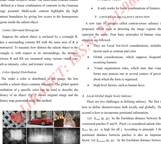
Contrast is the most commonly used local feature for attention detection because the contrast operator simulates the human visual receptive fields. The multi-scale contrast feature is defined as a linear combination of contrasts in the Gaussian image pyramid. Multi-scale contrast highlights the high contrast boundaries by giving low scores to the homogenous regions inside the salient object

B. Center-Surround Histogram

Suppose the salient object is enclosed by a rectangle R. Then a surrounding contour RS with the same area of R is constructed. To measure how distinct the salient object in the rectangle is with respect to its surroundings, the distance between R and RS are measured using various visual cues such as intensity, color, and texture/ texton.

C. Color-Spatial Distribution

The wider a color is distributed in the image, the less possible a salient object contains this color. The global spatial distribution of a specific color can be used to describe the saliency of an object. Fig. 2 shows original image and the saliency map generated using this method.

Fig. 3 Original image and saliency map

D. Advantage

 The method used is simple and fast.

E. Disadvantages

 Procedure detects only salient objects with rectangular shapes.

 It only works for linear combinations of features.

V. CONTEXT-AWARE SALIENCY DETECTION

A new type of saliency called context-aware saliency is proposed, which aims at detecting the image regions that represent the scene. Four basic principles of human visual attention are followed.

 They are Local low-level considerations, including factors such as contrast and color

 Global considerations, which suppress frequently occurring features

 Visual organization rules, which state that visual forms may possess one or several centers of gravity about which the form is organized.

 High-level factors, such as human faces.

A. Local-Global Single Scale Saliency

There are two challenges in defining saliency. The first is how to define distinctiveness both locally and globally. The second is how to incorporate positional information.

Let dcolor(pi ,pj) be the Euclidean distance between the

vectorized patches Piand Pj Pixel i is considered salient when

dcolor (pi, pj) is high for all j. According to principle 3 the

positional distance between patches is also an important factor. Let dposition(pi, pj) be the Euclidean distance between

image dimension. Based on the observations above a dissimilarity measure is defined between a pair of patches as:

, =_{1 + .} ( , )_{( , )}

Pixel i is considered salient when it is highly dissimilar to all other image patches, i.e., when (pi, pj) is high for all j.The

single-scale saliency value of pixel i at scale r is defined as

= 1 − −1 ( , )

B. Multi-Scale Saliency Enhancement

Background pixels (patches) are likely to have similar patches at multiple scales, e.g., in large homogeneous or blurred regions. This is in contrast to more salient pixels that could have similar patches at a few scales but not at all of them.

C. Including Immediate context

Areas that are close to the foci of attention should be explored significantly more than faraway regions. When the regions surrounding the foci convey the context, they draw our attention and thus are salient

D. High-level factors

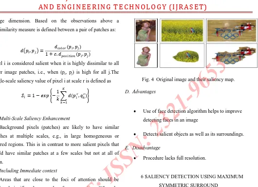
Finally, the saliency map should be further enhanced using some high-level factors, such as recognized objects or face detection. Face detection algorithm is incorporated, which generates 1 for face pixels and 0 otherwise. The saliency map is modified by taking the maximum value of the saliency map and the face map

Fig. 4 Original image and their saliency map.

D. Advantages

 Use of face detection algorithm helps to improve detecting faces in an image

 Detects salient objects as well as its surroundings.

E. Disadvantage

 Procedure lacks full resolution.

6 SALIENCY DETECTION USING MAXIMUM SYMMETRIC SURROUND

Detection of visually salient image regions is useful for applications like object segmentation, adaptive compression, and object recognition. If the salient regions comprise more than half the pixels of the image, or if the background is complex, the background gets highlighted instead of the salient object.

Fig. 5 Original images and their corresponging saliency map

A. Advantages

 Procedure is computationally efficient.

 It is easy to implement.

B. Disadvantage

 If the boundaries are not well defined, it will affect the accuracy of saliency map.

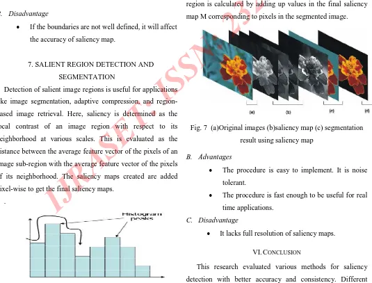
7. SALIENT REGION DETECTION AND SEGMENTATION

Detection of salient image regions is useful for applications like image segmentation, adaptive compression, and region-based image retrieval. Here, saliency is determined as the local contrast of an image region with respect to its neighborhood at various scales. This is evaluated as the distance between the average feature vector of the pixels of an image sub-region with the average feature vector of the pixels of its neighborhood. The saliency maps created are added pixel-wise to get the final saliency maps.

.

Fig. 6 Example of an image with acceptable resolution

A. Whole Object Segmentation Using Saliency Maps

The image is over-segmented using a simple K-means algorithm. The K seeds for the K-means segmentation are automatically determined using the hill-climbing algorithm in the three-dimensional CIELab histogram of the image. The number of peaks obtained indicates the value of K, and the values of these bins form the initial seeds. Once the segmented regions are found, the average saliency value V per segmented region is calculated by adding up values in the final saliency map M corresponding to pixels in the segmented image.

Fig. 7 (a)Original images (b)saliency map (c) segmentation result using saliency map

B. Advantages

 The procedure is easy to implement. It is noise tolerant.

 The procedure is fast enough to be useful for real time applications.

C. Disadvantage

 It lacks full resolution of saliency maps.

VI. CONCLUSION

saliency detection methods are analyzed during the research. Among them Qi Wang, Yuan Yuan Saliency Detection by Multiple-Instance Learning [1] have better saliency maps. Saliency map of [1] have better accuracy and consistent output.

ACKNOWLEDGMENT

The author acknowledge the reviewers and associate editor for constructive and useful feedback.

REFERENCES

[1] Qi Wang, Yuan Yuan, “Saliency Detection by Multiple

-Instance Learning,” IEEE transactions on cybernetics, vol. 43, no. 2, April 2013

[2] T. Liu, Z. Yuan, J. Sun, J. Wang, N. Zheng, X. Tang, and H.-Y. Shum, “Learning to detect a salient object,” IEEE Trans. Pattern Anal. Mach. Intell.,vol. 33, no. 2, pp. 353–367,Feb.2011

[3] S. Goferman, L. Zelnik-Manor, and A. Tal, “Context

-aware saliency detection,” Proc. IEEE Int. Conf.

Comput. Vis. Pattern Recognit, 2010, pp. 2376–2383. [4] A.Radhakrishna and S.Sabine,"Saliency Detection using

maximum Symmetric Surround Int.Conf.Image Process,2010,pp.2653-2656

[5] R. Achanta, F. J. Estrada, P.Wils, and S. Süsstrunk,

“Salient region detection and segmentation”,Proc.