Analysis of Reversed Trapezoidal Fins using a 2-D
Analytical Method
Hyung Suk Kang
Department of Mechanical and Biomedical Engineering, Kangwon National University, South Korea
Copyright © 2015 by authors, all rights reserved. Authors agree that this article remains permanently open access under the terms of the Creative Commons Attribution License 4.0 International License
Abstract
This paper presents a two-dimensional analysis of reversed trapezoidal fins with variable fin base thickness. Heat loss from the reversed trapezoidal fin is presented as a function of the fin shape factor, fin base thickness, and fin base height. The relationship between the fin tip length and the convection characteristic number, as well as that between the fin tip length and the fin base height for equal amounts of heat loss are analyzed. In addition, the relationship between the fin base thickness and the fin shape factor for equal amounts of heat loss is presented. One of the results shows that the heat loss decreases linearly with the increase in the fin shape factor.Keywords
Reversed Trapezoidal Fins, Fin Base Thickness, Fin Shape Factor, Convection Characteristic Number, Heat Loss1. Introduction
Extended surfaces or fins are well known to be simple and effective means of increasing heat dissipation in many engineering and industrial applications, such as the cooling of combustion engines, electronic equipments, and many kinds of heat exchangers. As a result, a great deal of attention has been directed to the fin problems, and many studies on the various shapes of fins have been presented. The most commonly studied fins are longitudinal rectangular, triangular, and trapezoidal fins and annular or circular fins. For example, Sen and Trinh [1] studied the rate of heat loss from a rectangular fin governed by the power law-type temperature dependence. Kang and Look [2] analyzed the trapezoidal fin with various lateral surface slopes while Yeh [3] investigated the optimum dimensions of rectangular fins and cylindrical pin fins. Kang and Look [4] presented the analysis of thermally asymmetric triangular fin using a two-dimensional analytical method. Sikka and Iqbal [5] made an analysis of the heat transfer characteristics of a circular fin dissipating heat from its surface by convection and radiation. Recently, Moitsheki et
al. [6] considered a model describing the temperature profile in a longitudinal fin with rectangular, concave, triangular and convex parabolic profiles by using optimal homotopy analysis method while Huang and Chung [7] determined the optimum shapes of partially wet annular fins adhered to a bare tube based on the desired fin efficiency and fin volume with the conjugate gradient method. In all these studies, fin base temperature is given as a constant for the fin base boundary condition.
The effect of the fin base thickness variation on fin performance is considered in some studies. For example, Abrate and Newnham [8] studied heat conduction in an array of triangular fins with an attached wall using the finite element method. Kang [9] presented an optimum procedure for geometrically asymmetric straight trapezoidal fins with variable fin base thickness in the case of fixed fin volumes.
In addition, studies on unique fin shapes have been reported. For example, Bejan and Almogbel [10] reported the geometric (constructal) optimization of T-shaped fin assemblies, where the objective is to maximize the global conductance of the assembly, subject to total volume and fin-material constraints while Hashizume et al. [11] analyzed fin efficiency of serrated fins and derived the theoretical fin efficiency in the form of a function of modified Bessel functions. Kundu and Das [12] analyzed and optimized elliptical disk fins using a semi-analytical technique.
In this study, reversed trapezoidal fins with variable fin base thickness are analyzed using a two-dimensional analytic method. The shapes of fins can be changed from rectangular fins to reversed trapezoidal fins with different lateral surface slopes by adjusting the fin shape factor. In this analysis, both the fin base thickness and the fin base height are varied. Therefore, the thermal resistance from the inside wall to the fin base is changed due to a variation in the fin base thickness, and the thermal energy source is varied with a variation in the fin base height.
The schematic diagram of a reversed trapezoidal fin is shown in Fig. 1. For this fin geometry, dimensionless two-dimensional governing differential equation under steady state is
0 2 2 2 2 = ∂ ∂ + ∂ ∂ Y X θ θ
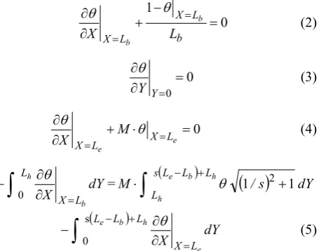
. (1) Three boundary conditions and one energy balance condition are required to solve the governing differential equation and these conditions are given as (2)-(5).
0 1 = − + ∂ ∂ = = b L X L X L
X b b
θ θ (2) 0 0 = ∂ ∂ = Y Y θ (3) 0 = ⋅ + ∂ ∂ = =Le X Le
X M X θ θ (4)
∫
∂ = ∂ − h b L L X dY X 0 θ=M
(
e b)
h( )
/s dYh
L L L s
L 1 1
2
∫
− + + ⋅ θ(
)
∫
− + ∂ = ∂− e b h
e L L L L X dY X s 0 θ (5)
A fin base boundary condition is represented by (2), which reveals that heat conduction from the inside wall to the fin base is equal to heat conduction through the fin base. Equation (3) is a fin center line condition, and it means that there is no heat transfer through the fin center line due to the symmetric geometry. Equation (4) is a boundary condition at the fin tip, showing that, physically, heat conduction to the tip surface equals the heat convection from that surface. The energy balance condition as given by (5) describes that the heat conduction through a fin base equals the sum of the heat loss from all of the fin surfaces. When (1) with three boundary conditions (2), (3) and (4) are solved, the temperature distribution θ(X, Y) within the reversed trapezoidal fin can be obtained using the separation of variables procedure. The result is
(
)
∑
∞( ) ( )
( )
( )
( )
= +
⋅ ⋅ =
1 2 3
1 cos
n n n
n n g g Y X f g Y ,
X λ λ λ λ
θ . (6)
where,
( )
X(
X)
g( )
(
X)
f =coshλn + 4 λn ⋅sinhλn (7)
( )
(
(
)
)
h h
n
h
n L L L
g
n n
1λ =2λ 4sin+sinλ 2λ (8)
( )
n(
Lb)
Lb n(
Lb)
g2 λ =coshλn − ⋅λ ⋅sinhλn (9)
( )
n g( )
n{
(
nLb)
nLb(
nLb)
}
g3λ = 4λ ⋅ sinhλ −λ ⋅coshλ (10)
( )
(
(
)
)
e n n e n nn M L LM
g λ λλ λ λ
tanh tanh
4 =− +⋅ ⋅ + (11)
The eigenvalues λn can be obtained using (12), which is an arranged form of (5).
0=g5
( )
λn −g6( )
λn +g7( ) ( )
λn[
{
g8 λn( )}
n{
g( )
n g( )
n g( )
ng9 λ ⋅ 10 λ + 11λ − 12 λ +
( )}
n{
g( )
n g( )
n}
{
g( )
ng13 λ + 14 λ + 15 λ ⋅ 16 λ −
( )
n g( )
n g( )}
n]
g17 λ − 18 λ − 19 λ
+ (12)
where,
( )
n{
(
nLb)
[image:2.595.72.300.209.388.2]g5λ = sinhλ +g4
( )
λn ⋅cosh(
λnLb)} (
sinλnLh)
(13)Figure 1. Geometry of a reversed trapezoidal fin
( )
n{
(
nLe)
g6 λ = sinhλ
( )
λ ⋅(
λ)}
{
λ(
−ξ)
}
+g4 n cosh nLe sin nLh 2 (14)
( )
2 7 1 s M g n n + ⋅ = λλ (15)
( )
− = s L L g h b n n8λ cosh λ (16)
( )
( )
− ⋅ = s L L gg9 λn 4 λn sinh λn b h (17)
( )
λ λ(
ξ)
⋅{
λ(
−ξ)
}
−
= 2 cos 2
s
sinh n n
10 n Lh Lh
g (18)
( )
λ λ(
ξ)
⋅{
λ(
−ξ)
}
− ⋅
= cosh n 2 sin n 2
11 n s sLh Lh
g (19)
( )
(
)
⋅ = s L Lg12 λn cosλn h sinh λn h
(20)
( )
(
)
⋅ ⋅ = s L L sg13 λn sinλn h cosh λn h
(21)
( )
− = s L L g h b n n( )
( )
− ⋅ = s L L g g h b nn 4 n
15 λ λ cosh λ (23)
( )
λ λ(
ξ)
⋅{
λ(
−ξ)
}
−= 2 cos 2
s
cosh n n
16 n Lh Lh
g (24)
( )
λ λ(
ξ)
⋅{
λ(
−ξ)
}
− ⋅
= sinh n 2 sin n 2
17 n s sLh Lh
g (25)
( )
(
)
⋅ = s L Lg18 λn cosλn h cosh λn h
(26)
( )
(
)
⋅ ⋅ = s L L sg n h
h
n λ λ
λ sin n sinh
19
(27)
The eigenfunction equation (12) is too long and complicated to obtain all the eigenvalues simultaneously. So the first eigenvalue, λ1, is directly obtained from (12) by using the incremental search method. The remaining eigenvalues (i.e., λ2, λ3, λ4, ∙∙∙) are calculated from (28) by using the Newton-Raphson method. Equation (28) is derived from the orthogonality principle used in the separation of variables method and is a modified form of the equation that is presented by Kang and Look [2].
(
n)
n λ λ
λ = 2 1+
(
)
(
)
(
(
)
)
h h
h
n L L L
n 1
n 1 tan tan tan
2λ λ λ λ λ
+ +
− (28)
Through the procedure of obtaining the rest eigenvalues (i.e.,
λ
2,λ
3,λ
4, ∙∙∙) from Eq. (28), the 2-D analytic method used in this study can be applied to many configurations of fins, such as, asymmetric straight trapezoidal fins, annular trapezoidal fins, straight parabolic fins, etc. The heat loss conducted into the fin through the fin base is calculated by∫
∂ = ∂ − = h b l w l x l dyx T k q
0
[image:3.595.81.298.81.243.2]2 . (29)
Table 1. The temperature ratio with the variations in NPY at X=Le.
(M=0.2, Lb=0.1, Le=2.1, Lh=0.5)
θ(NPY)/θ(NPY=0) (%)
NPY ξ=0 ξ=0.5 ξ=1
0.2 99.14 99.54 99.81
0.4 96.57 98.16 99.23
0.6 92.34 95.88 98.26
0.8 86.52 92.71 96.92
1.0 79.20 88.69 95.20
The dimensionless heat loss from the reversed trapezoidal fin is denoted by (30).
( ) ( )
( )
( )
∑
∞ = + ⋅ − = =1 2 3
5 1
2
n n n
n n w
i g g
g g l
k q
Q φ λλ λλ (30)
Fin efficiency is defined as the ratio of heat loss from the fin,
Q
to the ideal heat loss from the fin,Q
id and can be calculated by using Eq. (31).(
)
+ + − + = = s s L L L M Q Q Q b e h bid 2 θ 1 2
h
(31)
3. Results and Discussions
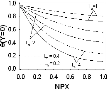
For two different fin base heights and three different fin tip lengths, the temperature profile along the fin centerline is represented in Fig. 2. The normalized position of X, NPX, is given as (X-Lb)/(Le-Lb) so that NPX=0 means the position at
the fin base and NPX=1 at the fin tip. As the fin base height increases from 0.2 to 0.4, the fin temperature along the fin centerline increases for all three values of Le. It can be
inferred that at the center of the fin tip, the difference between the temperature for Lh=0.2 and that for Lh=0.4
increases first and then decreases as the fin tip length increases from 1 to 4.
Figure 2. Dimensionless temperature profile along the normalized position of X (M=0.1, Lb=0.1, ξ=0.5)
Table 1 lists the temperature ratio with a variation in the normalized position of Y [i.e. NPY = Y/{(2-ξ)Lh}] at the fin
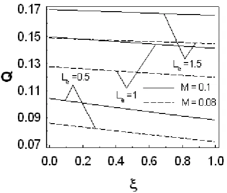
[image:3.595.320.546.340.531.2] [image:3.595.59.296.541.622.2]Figure 3. Heat loss as a function of the fin shape factor (Lb=0.1, Lh=0.1)
Figure 4. Heat loss as a function of the fin base thickness (M=0.1, ξ=0.5)
Figure 3 presents the dimensionless heat loss as a function of the fin shape factor for different values of the dimensionless fin tip length. As expected, the heat loss decreases as the fin shape factor increases due to the decrease in the fin surface area, and this phenomenon is more remarkable as the fin tip length decreases. Therefore, it can be inferred that the effect of ξ on heat loss disappears if the fin length is very long. It is observed that the heat loss decreases almost linearly with the increase in ξ for all given values of Le and M.
The effect of the dimensionless fin base thickness on heat loss is represented in Fig. 4. As expected, the fin base thickness has a significant influence on heat loss, because the fin base temperature decreases due to the increased thermal resistance as the fin base thickness increases. It shows that the heat loss decreases almost linearly as the fin base thickness increases, even though the actual fin length (i.e. Le
- Lb) remains constant. It also shows that the effect of the
fin base thickness on heat loss becomes a little more
[image:4.595.316.548.106.304.2]remarkable as the fin length increases from 1 to 2 for a fixed fin base height.
Figure 5. Heat loss as a function of the fin base height (ξ=0.5, Lb=0.1)
Figure 5 shows the dimensionless heat loss as a function of the dimensionless fin base height for two different fin lengths and three different convection characteristic numbers. For all given convection characteristic numbers, the heat loss increases a little more rapidly first and then increases linearly for Le-Lb=2, while it increases linearly for Le-Lb=0.5 as the
fin base height increases. It is noted that the effect of the convection characteristic number on heat loss becomes more remarkable as the fin base height increases. For example, in the case of Le-Lb=2, the heat loss increases from 0.1582 to
0.1947 (i.e., difference=0.0365 and ratio=1.23) at Lh=0.1,
while it increases from 0.4039 to 0.5397 (i.e., difference=0.1358 and ratio=1.34) at Lh=0.9 as M increases
[image:4.595.60.292.300.494.2]from 0.08 to 0.12.
Figure 6 shows the relationship between the fin tip length and the fin base height for equal amounts of heat loss based on the values of Le=0.8 and Lh=0.2 in the cases of M=0.01,
0.05 and 0.1. This shows that the fin length decreases parabolically as the fin height increases from 0.1 to 0.2 and then decreases linearly as the fin height increases from 0.2 to 0.3 in the case of M=0.1. It also shows that the fin length decreases linearly as the fin height increases from 0.1 to 0.3 in the case of M=0.01.
Figure 7 presents the relationship between the fin tip length and the convection characteristic number for equal amounts of heat loss based on the value of Le=2 and M=0.05
for three values of the fin shape factor. The value of Le
Figure 6. Relationship between the fin tip length and the fin base height for equal amounts of heat loss (ξ=0.5, Lb=0.1)
Figure 7. Relationship between the fin tip length and the convection characteristic number for equal amounts of heat loss (Lb=0.1, Lh=0.4)
The relationship between the fin base thickness and the fin shape factor for equal amounts of heat loss based on the values of Lb=0.2 and ξ =0.25 for three values of the fin
length is depicted in Fig. 8. The value of Lb decreases
almost linearly with an increase in ξ for all three of the fin length values. This shows that the variation in Lb with the
[image:5.595.60.293.306.500.2]variation in ξ becomes less remarkable as the fin length increases. From this phenomenon, it can be physically inferred that the fin shape has no effect on heat loss when the fin length is very long.
Figure 8. Relationship between the fin base thickness and the fin shape factor for equal amounts of heat loss (M=0.1, Lh=0.2)
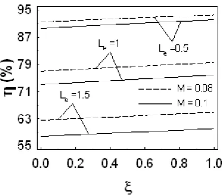
Figure 9. Fin efficiency as a function of the fin shape factor (Lb=0.1,
Lh=0.1)
[image:5.595.318.544.307.505.2]4. Conclusions
From this 2-D analysis of reversed trapezoidal fins, the following conclusions can be drawn:
1. Heat loss decreases linearly while the fin efficiency increases linearly as the fin shape factor increases.
2. Heat loss decreases as the fin base thickness increases, while it increases with an increase in the fin base height.
3. When other variables are fixed, the fin tip length decreases parabolically as the convection characteristic number increases for equal amounts of heat loss.
4. The fin base thickness decreases linearly with an increase in the fin shape factor, while the fin length decreases parabolically with an increase in the convection characteristic number for equal amounts of heat loss.
Nomenclature
h: heat transfer coefficient [W/m2℃]
k: thermal conductivity [W/m℃] lb: fin base thickness [m]
Lb: dimensionless fin base thickness, lb/lc
lc: characteristic length [m]
le: fin tip length [m]
Le: dimensionless fin tip length, le/lc
lh: one half fin base height [m]
Lh: dimensionless one half fin base height, lh/lc
lw: fin width [m]
q: heat loss from the fin [W]
Q
: dimensionless heat loss from the fin, q/(klwφi)s: fin lateral surface slope, {(1-ξ)lh}/(le-lb)
T: fin temperature [℃] Tb: fin base temperature [℃]
Ti: inside wall temperature [℃]
T∞: ambient temperature [℃]
x: fin length directional variable [m]
X: dimensionless fin length directional variable, x/lc
y: fin height directional variable [m]
Y: dimensionless fin height directional variable, y/lc
Greek Symbol
i
φ : adjusted temperature of the inside wall [℃], (Ti-T∞) h: fin efficiency
n
λ : eigenvalues (n = 1, 2, 3, ∙∙∙)
θ: dimensionless temperature, (T-T∞)/(Ti-T∞)
b
θ : dimensionless fin base temperature, (Tb-T∞)/(Ti-T∞)
ξ: fin shape factor, 1-s(le-lb)/lh, (0≤ξ≤1)
Subscript
b: fin base c: characteristic e: fin tip
h: fin base height i: inside wall id: ideal w: fin width
∞: ambient
REFERENCES
[1] A. K. Sen, S. Trinh, An exact solution for the rate of heat transfer from a rectangular fin governed by a power law-type temperature dependence, ASME J. of Heat Transfer, Vol. 108, No. 5, 457-459, 1986.
[2] H. S. Kang, D. C. Look, Jr., Two dimensional trapezoidal fins analysis, Computational Mechanics Vol.19, No. 3, 247-250, 1997.
[3] R. H. Yeh, An analytical study of the optimum dimensions of rectangular fins and cylindrical pin fins, Int. J. of Heat and Mass Transfer Vol. 40, No. 15, 3607-3615, 1997.
[4] H. S. Kang, D. C. Look, Jr., Thermally asymmetric triangular fin analysis, AIAA J. of Thermophysics and Heat Transfer Vol. 15, No. 4, 427-430, 2001.
[5] S. Sikka, M. Iqbal, Temperature distribution and effectiveness of a two-dimensional radiating and convecting circular fin, AIAA Journal Vol. 8, No. 1, 101-106, 1970. [6] R. J. Moitsheki, M. M. Rashidi, A. Basiriparsa, A. Mortezaei,
Analytical solution and numerical simulation for one-dimensional steady nonlinear heat conduction in a longitudinal radial fin with various profiles, Heat Transfer-Asian Research Vol. 44, No. 1, 20-38, 2015.
[7] C. H. Huang, Y. L. Chung, An inverse problem in determining the optimum shapes for partially wet annular fins based on efficiency maximization, Int. J. of Heat and Mass Transfer Vol. 90, 364-375, 2015.
[8] S. Abrate, P. Newnham, Finite element analysis of triangular fins attached to a thick wall, Computers and Structures Vol. 57, No. 6, 945-957, 1995.
[9] H. S. Kang, Optimization of geometrically asymmetric straight trapezoidal fins, Journal of Mechanical Science and Technology Vol. 28, No. 12, 5205-5212, 2014.
[10] A. Bejan, M. Almogbel, Constructal T-shaped fins, Int. J. of Heat and Mass Transfer Vol. 43, 2101-2115, 2000.
[11] K. Hashizume, R. Morikawa, T. Koyama, T. Matsue, Fin efficiency of serrated fins, Heat Transfer Engineering Vol. 23, No. 2, 6-14, 2002.