FUNCTIONAL LINK NEURAL NETWORK WITH
MODIFIED BEE-FIREFLY LEARNING
ALGORITHM FOR CLASSIFICATION TASK
YANA MAZWIN MOHMAD HASSIM
FUNCTIONAL LINK NEURAL NETWORK WITH MODIFIED BEE-FIREFLY LEARNING ALGORITHM FOR CLASSIFICATION TASK
YANA MAZWIN MOHMAD HASSIM
A thesis submitted in
fulfillment of the requirement for the award of the Doctor of Philosophy.
Faculty of Computer Science and Information Technology Universiti Tun Hussein Onn Malaysia
iii
ACKNOWLEDGEMENT
All praise to the almighty Allah, for the good health and wellbeing that were necessary to complete this study. I would like to express my sincere gratitude to Assoc. Prof. Dr. Rozaida Ghazali, my supervisor, for the continuous support of my PhD study and research, for her patience, motivation, enthusiasm, and immense knowledge. Her guidance helped me in all the time of research and writing of this thesis.
I take this opportunity to express gratitude to Faculty of Computer Science and Information Technology (FSKTM) and Centre for Graduate Studies (CGS) of Universiti Tun Hussein Onn Malaysia (UTHM) for providing good facilities and inspiring environment for me to complete this study.
iv
ABSTRACT
Classification is one of the most frequent studies in the area of Artificial Neural Network (ANNs). The ANNs are capable of generating a complex mapping between the input and the output space to form arbitrarily complex nonlinear decision boundaries. One of the best-known types of ANNs is the Multilayer Perceptron (MLP). MLP usually requires a large amount of available measures in order to achieve good classification accuracy. To overcome this, a Functional Link Neural
Networks (FLNN) which has a single layer of trainable connection weights is used. The single layer property of FLNN also make the learning algorithm used less complicated compared to MLP network. The standard learning method for tuning
v
ABSTRAK
Pengkelasan adalah salah satu kajian yang paling kerap dilakukan dalam bidang
Artificial Neural Networks (ANNs). ANNs mampu menjana pemetaan kompleks di
antara ruang input dan output untuk membentuk sempadan keputusan tidak linear yang kompleks. Salah satu model yang paling terkenal dalam ANNs adalah
Multilayer Perceptron (MLP). MLP biasanya memerlukan beberapa langkah yang
disediakan untuk mencapai ketepatan pengelasan yang baik. Untuk mengatasi masalah ini, Functional Link Neural Network (FLNN) sejenis rangkaian neural yang mempunyai hanya satu lapisan pemberat digunakan untuk menggantikan MLP. Sifat FLNN yang hanya mempunyai satu lapisan pemberat juga membuat algoritma pembelajaran yang digunakan untuk melatih rangkaian menjadi kurang rumit berbanding dengan rangkaian MLP. Kaedah pembelajaran piawai untuk mengemaskini pemberat FLNN adalah dengan menggunakan algoritma
backpropagation (BP). Namun begitu, algoritma BP mudah terperangkap di local
minima yang mana ianya memberi kesan kepada prestasi rangkaian FLNN. Kajian
vi
TABLE OF CONTENTS
DECLARATION ii
ACKNOWLEDGEMENT iii
ABSTRACT iv
ABSTRAK v
TABLE OF CONTENTS vi
LIST OF TABLES x
LIST OF FIGURES xiv
LIST OF SYMBOLS AND ABBREVIATIONS xvii
LIST OF PUBLICATIONS xix
CHAPTER 1 INTRODUCTION 1
1.1 Background of Research 1
1.2 Problem Statements 3
1.3 Aim and Objective of Research 6
1.4 Scope of Research 6
1.5 Significance of Research 7
1.6 Chapter Summary 7
1.7 Organization of Thesis 7
CHAPTER 2 LITERATURE REVIEW 9
2.1 Introduction 9
2.2 Classification Task 10
vii
2.3.1 Components of Artificial Neural Networks 15 2.3.2 Different Models of Neural Networks 18
2.3.3 Feedforward Neural Networks 19
2.3.4 Multilayer Perceptron 20
2.4 Higher Order Neural Networks 22
2.4.1 Properties of HONNs 23
2.4.2 Types of HONNs 28
2.4.3 Functional Link Neural Networks (FLNN) 31
2.4.4 The FLNN Learning Algorithm 35
2.5 Swarm Intelligence Optimization 37
2.5.1 Artificial Bee Colony Algorithm 40
2.5.2 Firefly Algorithm 46
2.6 Hybridization of Metaheuristic Algorithms 49 2.7 Discussion: Scenario Leading to the Research
Framework 50
2.8 Chapter Summary 53
CHAPTER 3 RESEARCH METHODOLOGY 54
3.1 Introduction 54
3.2 Research Framework 54
3.2.1 Phase 1: Data Preparation 56
3.2.2 Phase 2: FLNN Training Procedure 65
3.2.3 Phase 3: Results Analysis 69
3.3 Environment 71
3.4 Parameters Setting 71
3.4.1 BP-learning Algorithm 71
3.4.2 ABC Learning Algorithm 72
3.4.3 MABC Learning Algorithm 73
3.4.4 MBF Learning Algorithm 74
3.5 Chapter Summary 75
CHAPTER 4 MODIFIED BEE-FIREFLY LEARNING ALGORITHM 76
4.1 Introduction 76
4.2 FLNN as objective function 77
viii
4.3.1 Initialization Phase 81
4.3.2 Employed Bees Phase 81
4.3.3 Onlooker Bees Phase 83
4.3.4 Scout Bees Phase 84
4.3.5 Pilot Experiment on FLNN-ABC 85 4.4 Modified ABC Learning Algorithm for FLNN
(FLNN-MABC) 93
4.4.1 Initialization Phase 98
4.4.2 Modified Employed Bees Phase 98 4.4.3 Modified Onlooker Bees Phase 98
4.4.4 Modified Scout Bees Phase 99
4.4.5 Experimentation on FLNN-MABC 100 4.5 Modified Bee-Firefly Learning Algorithm for
FLNN (FLNN-MBF) 104
4.5.1 Initialization Phase 107
4.5.2 Modified Employed Bees Phase 108
4.5.3 Onlooker Fireflies Phase 109
4.5.4 Modified Scout Bee Phase 110
4.6 Chapter Summary 113
CHAPTER 5 SIMULATION RESULTS AND DISCUSSION 114
5.1 Introduction 114
5.2 Experimental Design 114
5.2.1 Dataset Division 115
5.2.2 Network Model Topology 115
5.3 Best Average Simulation Results 116
5.4 Analysis of Results based on Datasets 123 5.4.1 Results of Proposed FLNN-MBF Model
with Standard FLNN-BP and MLP-BP
Models 123
5.4.2 Results on Improved Performance of
FLNN 127
5.4.3 Classification Performance of Proposed
ix
5.5 Statistical Performance Evaluation 138
5.6 Threat to Validity 139
5.7 Chapter Summary 140
CHAPTER 6 CONCLUSION AND FUTURE WORK 142
6.1 Introduction 142
6.2 Research Summary 142
6.3 Contribution 146
6.4 Future Works 146
6.5 Closing Remarks 148
REFERENCES 149
x
LIST OF TABLES
Table 2.1: FLNN application with BP-learning algorithm 36 Table 2.2: Properties of self-organization in swarms (Bonabeau
et al., 1999) 38
Table 2.3: The main components of honey bee swarms
(Karaboga, 2005) 41
Table 2.4: Application areas of ABC algorithm 44 Table 2.5: Applications of FA algorithms 48
Table 3.1: Summary of datasets 60
Table 3.2: Summary of missing value information in datasets 61
Table 3.3: Datasets after data cleaning 62
Table 3.4: Parameters setting in BP-learning algorithm 72 Table 3.5: Parameters setting in ABC learning algorithm 73 Table 3.6: Parameters setting in MABC learning algorithm 73 Table 3.7: Parameters setting in MBF learning algorithm 74 Table 4.1: Experimental result on XOR dataset 86 Table 4.2: Experimental result on 3-bit Parity problem 87 Table 4.3: Experimental result on 4-bit Encoder-Decoder
problem 88
Table 4.4: Pilot Experimental result on Balance Scale dataset
dataset 89
Table 4.5: Pilot Experimental result on Haberman’s Survival
dataset 89
Table 4.6: Pilot Experimental result on Mammographic Mass
Dataset 89
Table 4.7: Pilot Experimental result on Breast Cancer
Wisconsin (Original) Dataset 89
xi
Table 4.9: Pilot Experimental result on ILPD (Indian Liver
Patient Dataset) Dataset 90
Table 4.10: Pilot Experimental result on Iris Dataset 90 Table 4.11: Pilot Experimental result on Liver Disorders
(BUPA) Dataset 90
Table 4.12: Pilot Experimental result on Lymphographic
Dataset 91
Table 4.13: Pilot Experimental result on MONK's Problems
Dataset (MONK-2) 91
Table 4.14: Pilot Experimental result on Page Blocks
Classification Dataset 91
Table 4.15: Pilot Experimental result on Zoo Dataset 91 Table 4.16: Pilot Experimental result on Pima Indians Diabetes
Dataset 92
Table 4.17: Pilot Experimental result on Thyroid Disease
Dataset 92
Table 4.18: Binomial/binary classification datasets 101 Table 4.19: Multiclass classification datasets 101 Table 5.1: Best Average Result from MLP-BP 116 Table 5.2: Best Average Result from FLNN-BP 117 Table 5.3: Best Average Result from FLNN-ABC 117 Table 5.4: Best Average Result from FLNN-MABC 118 Table 5.5: Best Average Result from FLNN-MBF 118 Table 5.6: Number of trainable weights and biases used in all
network models 120
Table 5.7: Result of the proposed FLNN-MBF with standard models of FLNN-BP and MLP-BP on Balance
Scale dataset 123
Table 5.8: Result of the proposed FLNN-MBF with standard models of FLNN-BP and MLP-BP on Haberman’s
Survival dataset 123
Table 5.9: Result of the proposed FLNN-MBF with standard models of FLNN-BP and MLP-BP on
xii
Table 5.10: Result of the proposed FLNN-MBF with standard models of FLNN-BP and MLP-BP on Breast
Cancer Wisconsin dataset 124
Table 5.11: Result of the proposed FLNN-MBF with standard models of FLNN-BP and MLP-BP on Credit
Approval dataset 124
Table 5.12: Result of the proposed FLNN-MBF with standard
models of FLNN-BP and MLP-BP on ILPD dataset 124 Table 5.13: Result of the proposed FLNN-MBF with standard
models of FLNN-BP and MLP-BP on Iris dataset 125 Table 5.14: Result of the proposed FLNN-MBF with standard
models of FLNN-BP and MLP-BP on BUPA liver
disorders dataset 125
Table 5.15: Result of the proposed FLNN-MBF with standard models of FLNN-BP and MLP-BP on
Lymphographic dataset 125
Table 5.16: Result of the proposed FLNN-MBF with standard models of FLNN-BP and MLP-BP on MONK's
problems dataset 125
Table 5.17: Result of the proposed FLNN-MBF with standard models of FLNN-BP and MLP-BP on Page Blocks
Classification dataset 126
Table 5.18: Result of the proposed FLNN-MBF with standard
models of FLNN-BP and MLP-BP on Zoo dataset 126 Table 5.19: Result of the proposed FLNN-MBF with standard
models of FLNN-BP and MLP-BP on Pima
Indians diabetes dataset 126
Table 5.20: Result of the proposed FLNN-MBF with standard models of FLNN-BP and MLP-BP on Thyroid
disease dataset 126
Table 5.21: The overall improvement of FLNN-MBF 133 Table 5.22: Classification performance measurements in
xiii
Table 5.23: Classification performance measurements in
Haberman’s survival dataset 134
Table 5.24: Classification performance measurements in
mammographic mass dataset 134
Table 5.25: Classification performance measurements in Breast
Cancer Wisconsin dataset 134
Table 5.26: Classification performance measurements in Credit
Approval dataset 135
Table 5.27: Classification performance measurements in ILPD
dataset 135
Table 5.28: Classification performance measurements in Iris
dataset 135
Table 5.29: Classification performance measurements in BUPA
dataset 135
Table 5.30: Classification performance measurements in
Lymphographic dataset 136
Table 5.31: Classification performance measurements in
MONK's problems dataset 136
Table 5.32: Classification performance measurements in Page
Blocks Classification dataset 136
Table 5.33: Classification performance measurements in Zoo
dataset 136
Table 5.34: Classification performance measurements in Pima
Indians diabetes dataset 137
Table 5.35: Classification performance measurements in
Thyroid disease dataset 137
Table 5.36: Rank of each models on different dataset based on
classification accuracy 138
Table 5.37: Post-hoc procedure based on pairwise comparisons
xiv
LIST OF FIGURES
Figure 2.1: The input-output mapping of a classifier 10 Figure 2.2: Neuron and its representation (Samarasinghe, 2006) 16 Figure 2.3: Computational elements in artificial neuron 17
Figure 2.4: The basic structure of MLP 21
Figure 2.5: Inputs of neuron in first order neural network 24 Figure 2.6: Different architecture of HONNs (Ghazali, 2007) 25
Figure 2.7: Truth table for XOR problem 26
Figure 2.8: Solving XOR problem by using 2nd order HONN 26 Figure 2.9: Linear separation hyperplane for XOR problem
using 2nd order HONN 27
Figure 2.10: The architecture of FLNN 28
Figure 2.11: Pi Sigma Neural Network of K-th order 29 Figure 2.12: The Ridge Polynomial Neural Network of k-th
order 30
Figure 2.13: The FLNN of type functional expansion model 32 Figure 2.14: The FLNN of type tensor representation 33 Figure 2.15: The standard ABC pseudo code 43 Figure 2.16: The standard FA pseudo code 48 Figure 2.17: Scenario Leading to the Research Framework 52
Figure 3.1: The research framework 55
Figure 3.2: Pictorial representation of 10-fold cross-validation 64 Figure 3.3: The influence of learning rate on network learning 67 Figure 4.1: The development process of proposed learning
algorithm 77
xv
Figure 4.4: Exploitation process and food positions visualized
by the employed bee 82
Figure 4.5: The greedy selection 82
Figure 4.6: Exploitation process and food positions visualized
by the onlooker bee 83
Figure 4.7: Exploration by scout bee 84
Figure 4.8: Pseudo code of the ABC learning algorithm for
FLNN 85
Figure 4.9: Truth table for 3-bit Parity problem 87 Figure 4.10: Truth table for 4-bit Encoder-Decoder problem 88 Figure 4.11: Exploitation process of employed and onlooker
bee in MABC algorithm 95
Figure 4.12: Global exploration of scout bee in MABC
algorithm 95
Figure 4.13: Flowchart of MABC learning algorithm for FLNN 97 Figure 4.14: Pseudo code of the MABC learning algorithm for
FLNN 100
Figure 4.15: Experimental results on binomial/binary
classification datasets 102
Figure 4.16: Experimental results on multiclass classification
datasets 103
Figure 4.17: The main step of the proposed MBF algorithm 106 Figure 4.18: Pseudo code of the MBF learning algorithm for
FLNN 111
Figure 4.19: Flowchart of MBF learning algorithm for FLNN 112 Figure 5.1: Best accuracy results from all network models 119 Figure 5.2: FLNN performance on NMSE with increasing
network order 121
Figure 5.3: MLP performance on NMSE with increasing
hidden nodes 122
Figure 5.4: Classification accuracy of FLNN network trained
xvi
Figure 5.5: Classification accuracy of FLNN network trained with different algorithms in Haberman’s Survival
dataset 128
Figure 5.6: Classification accuracy of FLNN network trained with different algorithms in the mammographic
mass dataset 128
Figure 5.7: Classification accuracy of FLNN network trained with different algorithms in the Breast Cancer
Wisconsin dataset 128
Figure 5.8: Classification accuracy of FLNN network trained
with different algorithms in Credit Approval dataset 129 Figure 5.9: Classification accuracy of FLNN network trained
with different algorithms in ILPD dataset 129 Figure 5.10: Classification accuracy of FLNN network trained
with different algorithms in Iris dataset 129 Figure 5.11: Classification accuracy of FLNN network trained
with different algorithms in BUPA dataset 130 Figure 5.12: Classification accuracy of FLNN network trained
with different algorithms in Lymphographic dataset 130 Figure 5.13: Classification accuracy of FLNN network trained
with different algorithms in MONK's problems
dataset 130
Figure 5.14: Classification accuracy of FLNN network trained with different algorithms in Page Blocks
Classification dataset 131
Figure 5.15: Classification accuracy of FLNN network trained
with different algorithms in Zoo dataset 131 Figure 5.16: Classification accuracy of FLNN network trained
with different algorithms in Pima Indians diabetes
dataset 131
Figure 5.17: Classification accuracy of FLNN network trained
xvii
LIST OF SYMBOLS AND ABBREVIATIONS
𝑤 - Connection weight
𝑓(𝑥), 𝜎 - Activation function
𝐷 - Dimensions
𝐸 - Network error
𝑥 - The input vector
𝑌 - Network output
𝑌̂ - Target output/ Desired output
1 1 + 𝑒−𝑥
- Logistic sigmoid function
tanh (𝑥) - Hyperbolic tangent
𝜀 - Learning rate
𝜇 - Momentum coefficient
П - product term
Σ - summation function
𝐿𝐵 - Lower bound
𝑈𝐵 - Upper bound
𝑆𝑁 - Solutions number
𝑇𝑃 - True Positives
𝑇𝑁 - True Negatives
𝐹𝑃 - False Positives
𝐹𝑁 - False Negatives
𝑙𝑖𝑚𝑖𝑡 - Local search abandonment limit
𝛽0 - Initial attractiveness
𝛾 - Light absorption coefficient
ABC - Artificial Bee Colony
ANNs - Artificial Neural Networks
xviii
DE - Differential evolution
FA - Firefly Algorithm
FLNN - Functional Link Neural Network
GA - Genetic Algorithm
HONNs - Higher-order Neural Networks
MAE - Mean absolute error
MLP - Multilayer Perceptron
MABC - Modified Artificial Bee Colony
MBF - Modified Bee-Firefly
MSE - Mean square error
NMSE - Normalized mean squared error
PSNN - Pi-Sigma Neural Network
PSO - Particle Swarm Optimization
RMSE - Root mean squared error
RPNN - Ridge Polynomial Neural Network
SI - Swarm Intelligence
xix
LIST OF PUBLICATIONS
Journals:
(i) Yana Mazwin Mohmad Hassim and Rozaida Ghazali, “Training A Functional Link Neural Network using Artificial Bee Colony for a Classification Problems” Journal of Computing Press, NY, USA,
ISSN(online)2151-9617, volume 4, issue 9, 2012 (pp.110-115).
(ii) Yana Mazwin Mohmad Hassim and Rozaida Ghazali, “Using Artificial Bee Colony to improve Functional Link Neural Network Training”, Applied
Mechanics and Materials, ISSN 1662-7482, TTP USA, volume 263, 2013
(p.p 2102-2108).
(iii) Yana Mazwin Mohmad Hassim and Rozaida Ghazali, “An Approach to improve Functional Link Neural Network Training using Modified Artificial Bee Colony for Classification Task” , Asia-Pacific Journal of
Information Technology and Multimedia, e-ISSN: 2289-2192 volume 2,
issue 2, 2013 (pp. 63-71).
(iv) Yana Mazwin Mohmad Hassim and Rozaida Ghazali, “An Improved Functional Link Neural Network Learning Using Artificial Bee Colony Optimisation for Time Series Prediction”, Int. J. Business Intelligence and
Data Mining, ISSN(online) 1743-8195 ISSN 1743-8187, Vol. 8, No. 4,
xx
Proceedings:
(i) Yana Mazwin Mohmad Hassim and Rozaida Ghazali (2013). Solving a classification task using Functional Link Neural Networks with modified Artificial Bee Colony. 2013 Ninth International Conference on Natural
Computation (ICNC), IEEE.
(ii) Yana Mazwin Mohmad Hassim and Rozaida Ghazali (2013). Functional Link Neural Network–Artificial Bee Colony for Time Series Temperature Prediction. Computational Science and Its Applications–ICCSA 2013, Springer Berlin Heidelberg: 427-437.
(iii) Yana Mazwin Mohmad Hassim and Rozaida Ghazali (2014). A Modified Artificial Bee Colony Optimization for Functional Link Neural Network Training. Proceedings of the First International Conference on Advanced
Data and Information Engineering (DaEng-2013), Springer Singapore:
69-78.
(iv) Yana Mazwin Mohmad Hassim and Rozaida Ghazali (2014). Optimizing Functional Link Neural Network Learning Using Modified Bee Colony on Multi-class Classifications. Advanced in Computer Science and its
Applications, Springer Berlin Heidelberg: 153-159.
(v) Yana Mazwin Mohmad Hassim, Rozaida Ghazali and Noorhaniza Wahid (2014). Modified Bee-Firefly Algorithm for Training Functional Link Neural Network. The 3rd International Conference on Computer
Engineering & Mathematical Sciences (ICCEMS 2014), 4-5 December
1CHAPTER 1
INTRODUCTION
1.1 Background of Research
Classification is a process of categorizing objects which mostly involved in decision-making activity. It is one of the most frequent studies in the area of Artificial Neural Networks (ANNs) (Zhang, 2000; Misra and Dehuri, 2007; Chen et al., 2011; Al-Jarrah and Arafat, 2015; Mason, 2015). Classification is defined as a task of identifying and assigning an object to a predefined group based on a number of observed attributes related to that object. Solving a classification problem required a set of example records which called a training set that needs to be presented to the ANNs network so that the network can “learn” the pattern. Each record in the
2
In the field of Machine Learning (ML), ANNs is known as a family of statistical learning algorithm inspired by the way of human brain process information (Michalski et al., 2013). They are data driven self-adaptive method, in which they can change their structure based on external or internal information that flows through the network to model complex relationships between inputs and outputs. The recent vast research activities in neural classification have established that ANNs are a promising tool and have been widely applied to various real world classification task especially in industry, business and science (Zhang, 2000; Liao and Wen, 2007;
Hema et al., 2008; Al-Shayea, 2011; Ghazali et al., 2011; Yeatman et al., 2014;
Al-Jarrah and Arafat, 2015). One of the best-known types of ANNs is the Multilayer Perceptron (MLP). The application of MLP in classification tasks has shown better performance in comparison to the statistical method due to their nonlinear nature and training capability (Murtagh, 1991; Walde et al., 2004; Silva et al., 2008; Zabidi et al., 2010).
Despite the development of various types of ANNs, this research work examines the ability of Higher Order Neural Networks (HONNs) which focusing on Functional Link Neural Network (FLNN) for solving classification problems. FLNN is a class of HONNs that can perform nonlinear mapping by using only single layer of units (Giles and Maxwell, 1987). HONNs utilize higher order terms to expand their input space into higher dimensional space to achieve nonlinear separability which reduced the complexity of the network. The single layer property of FLNN also makes the learning algorithm used in the network less complicated as compared to other standard feedforward neural networks (Misra and Dehuri, 2007).
3
gradient descent optimization method has several drawbacks that can affect the performance of the neural network model (Haring et al., 1997; Sierra et al., 2001; Abu-Mahfouz, 2005; Dehuri et al., 2008). Therefore, this research emphasizes on improving the FLNN network learning algorithm for classification task by using Swarm Intelligence (SI) optimization techniques to overcome such drawback.
Neural networks and swarm intelligence methodologies have been proven effective in solving certain classes of problems. Neural Networks are good at mapping the input vector to outputs while Swarm Intelligence (SI) is very good at optimization task (Kennedy and Eberhart, 2001). It is expected in this work that, the optimization of network learning by using the SI method may overcome the standard gradient-based learning algorithm drawbacks. SI method is concerned with the design of intelligent multi-agent systems inspired by the collective behavior of social insects such as ant or bees as well as an animal society such as a flock birds or a school of fish (Blum and Li, 2008). Numerous well-known methods of SI are; Particle Swarm Optimization (PSO), Artificial Bee Colony Algorithm (ABC), Differential Evolution (DE), Evolutionary Algorithm (EA) and recently Firefly Algorithm (FA). ABC algorithm is known to have good exploration capabilities for their global search strategy (Zhu and Kwong, 2010). On the other hand, FA is renowned for having good ability in local search exploitation strategy (Fister et al., 2013; Bacanin and Tuba, 2014). Hence, this research work came with the interest to integrate ABC and FA algorithms so that the benefit from the advantage of both methods can be utilized to recover the gradient based learning drawbacks for training the FLNN network model.
1.2 Problem Statements
4
approximate any function as well as estimating posterior probabilities which provide the basis for establishing classification rule (Richard and Lippmann, 1991; Zhang, 2000).
One of the best-known types of ANNs is the Multilayer Perceptron (MLP). The MLP is a feedforward multilayered structured model and has been successfully applied in a broad class of classification tasks (Murtagh, 1991; Zhang et al., 1999; Zhang, 2000; Silva et al., 2008; Zabidi et al., 2010). The multilayer structure of MLP gives the network the ability to map both linear and non-linear relationship with a condition that, they are provided with a sufficient number of nodes and layers. Beside of it successfulness, MLP adopts computationally intensive training algorithms and introduces many local minima in the error surface (Yu, 2005; Parappa and Singh, 2013). In order to achieve good classification ability, MLP also requires a rather large amount of available measures; as to determine the appropriate number of neurons in layers and to fix a suitable number of hidden layers in its structure. Furthermore, as the number of hidden layers and nodes in MLP structure increases, the network architecture becomes more complex and training the network becomes more challenging. MLP networks with a large number of hidden layers and nodes also mean that they are having a large number of learning parameters. This may also affect the MLP performance as the network with a large number of learning parameters tend to memorize the training data which may lead to over-fitting and poor generalization (Lawrence and Giles, 2000).
To overcome the MLP drawbacks, a Functional Link Neural Network (FLNN) is considered in this study which has the ability to perform nonlinear mapping by using only single layer units (Pao, 1989). FLNN is a type HONNs that utilized a higher combination of it inputs and has certain advantages over MLP.
5
network training and widely utilized in conjunction with gradient descent optimization method.
Although BP-learning is the most used algorithm for training the FLNN network, the algorithm however, has several limitations which affect the performance of the FLNN with BP-learning (FLNN-BP) model. FLNN-BP tends to easily get trapped in local minima especially for those with highly non-linearly separable classification problems which is an inherent problem that exists in the BP-learning algorithm. The employment of BP-BP-learning algorithm as BP-learning algorithm
has made FLNN-BP model strictly depends on the shape of the error surface and since a common error surface may have many local minima and multimodal, this has typically made the FLNN-BP model prone to stuck in some local minima when moving along the error surface during the training phase. In addition, FLNN-BP model also very dependent on the choices of initial values of the weights as well as the parameters of the algorithm such as the learning rate and momentum which make it not very easy to meet the desired convergence criterion during the network training. Ismail, (2001) detailed that with proper learning algorithm FLNN may possess high learning capabilities that require less memory in terms of weights and nodes when compared to the MLP for similar performance levels. Therefore, further investigations to improve learning algorithm in FLNN are still desired.
6
strategy (Fister et al., 2013; Bacanin and Tuba, 2014). In SI optimization method, both exploration and exploitation are necessary and contradict to each other. In order to achieve good performances, the two abilities should be well balanced. Thus, in conjunction with the benefits of both ABC algorithm (exploration) and firefly algorithm (exploitation), this research intends to propose an improved learning algorithm named: Modified Bee-Firefly (MBF) algorithm to be used for training the FLNN network for the task of classification.
1.3 Aim and Objective of Research
The aim of the research is to design and implement an improved learning algorithm by using an Modified Bee-Firefly algorithm for training the FLNN for the task of classification. In order to achieve the research aim, a few objectives have been set:
(i) to propose an improved learning algorithm for FLNN using ABC optimization algorithm for classification tasks
(ii) to enhance (i) by removing random dimension selection in order to deal with issues in tuning the FLNN weights parameters
(iii) to incorporate Firefly algorithm with (ii) in order to improve its classification accuracy
(iv) to evaluate and compare the out-of-sample performance (iii) with ordinary FLNN and ordinary MLP based on classification performance
1.4 Scope of Research
7
1.5 Significance of Research
FLNN-MBF is important to be used in this research for the task of classification. This research may help in introducing an improved learning algorithm for training the FLNN network that may contribute to better classification performance.
1.6 Chapter Summary
There have been many ANNs applications and techniques developed for the task of classifications in the past. Several methods related to ANNs particularly have been investigated and carried out. However, the ordinary feedforward ANNs, which is the MLP, is prone to easily get stuck into local minima. Limitation such as network complexity of the models also makes the existing system less desirable for some applications. Thus, to overcome the drawbacks, this research focuses on utilizing FLNN model for the task of classification. FLNN has a simple architecture that reduces the learning complexity as compared to other feedforward networks. However, during network training FLNN tends to easily get trapped in local minima especially for those non-linearly separable classification problems, which is an inherent problem that exists in the BP-learning algorithm. Thus, an improved learning algorithm for FLNN is proposed in this study. The next chapter will discuss the literature on the existing ANNs and FLNN approaches related to the classification task, the network structure, and the learning algorithm being used for network training.
1.7 Organization of Thesis
8
2CHAPTER 2
LITERATURE REVIEW
2.1 Introduction
10
2.2 Classification Task
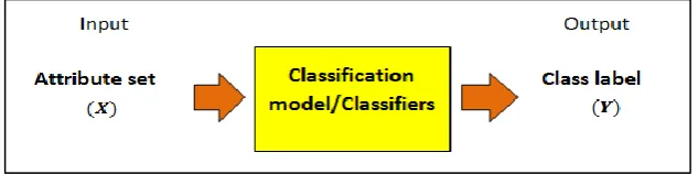
[image:30.595.161.478.398.477.2]Classification is the task of assigning objects to one of the several predefined categories and mostly involved in decision-making activity. Some examples of classification tasks include; assigning a given email into "spam" or "non-spam" classes and categorizing cells as malignant or benign based on the results of MRI scans. A classification problem occurs when an object needs to be assigned to a predefined group or class based on a number of observed attributes related to that object (Zhang, 2000). Bandyopadhyay et al. (2004), viewed a classification as an integral part of pattern recognition which involved dealing with a problem of generating appropriate class boundaries that can successfully distinguish various classes in the feature space. A system or classification models that implement classification are known as classifiers. The term "classifier" sometimes also refers to the mathematical function, implemented by a classification algorithm that maps input data to its class label.
Figure 2.1: The input-output mapping of a classifier
Figure 2.1 presents a classification as a task of mapping input attribute 𝑋 into its class label of 𝑌. The input data for a classification task is a collection of records. Each record, also known as an instance or example is characterized by a tuple 〈𝑋: 𝑌〉, where 𝑋 is the attribute set and 𝑌 is a special attribute, designated as the class label also known as category or target attribute. A tuples 𝑋 is represented by 𝑛 -dimensional attribute vector, where 𝑋 = {𝑥1, 𝑥2, … , 𝑥𝑛}, depicting 𝑛 measurements made on tuple from 𝑛 database attributes.
11
records it has not previously seen before. A general approach to solve a classification problem is by presenting a set of example pairs are known as training set which consists of an input attributes and class label to the classifier. The aim is to build a functional relationship between the class label (output) and attributes (input) to capture patterns in data through an iterative learning process devised by a learning algorithm (Rani, 2011). The learning algorithm analyzes the training data and produces an inferred function, which can be used for mapping new examples (test set).
Several methods have been taken toward a classification task which can be categorized into statistical methods and machine learning methods. Statistical methods are generally characterized by having an explicit underlying probability model, which provides a probability of being in each class rather than simply a classification (Michie et al., 1994). Traditional statistical classification methods usually try to find a clear cut boundary to divide the pattern space into some classification regions based on some predefined criterion (Li et al., 2002). Statistical pattern classification approach such as discriminant analysis is built based on Bayesian decision theory (Duda et al., 1995). In these methods, an underlying probability model must be assumed in order to calculate the posterior probability upon which the classification decision is performed.
In traditional statistical pattern classification method, the classifiers construct the model of class-conditional densities and build their decision based on the posteriors probability which is computed using the class-conditional likelihoods (Valous and Sun, 2012). Likelihoods are assumed to either come from a given probability density family, or a mixture of such densities or be written in a completely non-parametric way (Mahmoud et al., 2004). Bayes decision theory then allows choosing the class that minimizes the decision risk. The parameters of the densities are estimated to maximize the likelihood of the given sample for that particular class.
12
knowledge of both data properties and model capabilities before the models can be successfully applied (Dehuri and Cho, 2010).
In order to avoid limitations of classical statistical classification models, some researchers have turned their attention to machine learning methods. Machine learning is a subfield of computer science that evolved from the study of pattern recognition and computational learning theory in artificial intelligence. Machine learning aims to generate classifying expressions simple enough to be understood easily by the human (Donald et al., 1994). These methods have emerged as an important tool for classification as they are often capable of solving problems, which are not easily solvable by statistics models (Popelka et al., 2012). In machine learning, classification is considered an instance of supervised learning where a training set of correctly identified observations is available. Several prominent supervised machine learning methods include; decision trees, Support Vector Machine (SVM), and Artificial Neural Network (ANNs).
Decision tree learning is a method for approximating discrete-valued target functions, in which the learned function is represented by a decision tree (Zhang and Lee, 2003). Learned trees can also be represented as a set of if-then rules to improve human readability. The goal of decision tree learning is to create a model that predicts the value of a target variable based on several input variables. Decision tree learning methods are among the most popular inductive inference algorithms and have been successfully implemented in a broad range of tasks. However, the method can create over-complex trees that, does not generalize well from the training data. Also, there are certain concepts that are hard to learn and difficult to express when using decision trees representation such as XOR, parity or multiplexer problems. In such cases, the decision tree may become prohibitively large.
13
applicable for two-class classification tasks. Therefore, algorithms that can reduce the multi-class task into several binary problems are required for the SVM model.
Another widely used machine learning method is the artificial neural network (ANNs) models. ANNs is inspired by the structure and functional aspects of biological neural networks. The models are presented as systems of interconnected "neurons" which exchange messages between each other. The connections have numeric weights that can be tuned based on experience, making the neural nets adaptive to inputs and capable of learning. ANNs are non-linear statistical data modeling tools and are usually used to model complex relationships between inputs and outputs, to find patterns in data, or to capture the statistical structure in an unknown joint probability distribution between observed variables.
According to Zhang (2000), ANNs appears as a promising alternative methodology to various conventional classification methods based on three theoretical aspects; first, they are data-driven self-adaptive methods in which the system can adjust themselves to the data without any explicit specification of functional or distributional form to build the model. Second, they are universal functional approximators that can approximate any function with arbitrary accuracy and have more general and flexible functional forms than the traditional statistical method (Cybenko, 1989; Hornik, 1991). Since a classification task seeks a functional relationship between group membership and the attributes of the object, accurate identification of this function is important and neural networks method is well suited for such tasks (Zhang, 2000). And third, neural networks are a type of nonlinear models, which makes them flexible in modeling real world complex relationships and therefore, provides a robust foundation for establishing classification rules (Richard and Lippmann, 1991).
14
when involving with a highly complex nonlinear problem is still remain actively explored (Chen and Leung, 2004; Ghazali, 2007).
2.3 Artificial Neural Networks
Artificial Neural Networks (ANNs) is a computational information processing models that are inspired by human neural systems. ANNs mimic the structure of the biological central nervous system that could perform “Intelligent” task similar to
those performed by the human brain. According to Haykin (2004), the ANNs resembles the brain in two ways; 1) the knowledge is required by the network through a learning process and 2) the interneuron connection strength known as the synaptic weights are used to store the knowledge.
ANNs are generally presented as a system of interconnected neurons which can compute values from inputs and incrementally learn from their environment (data) to capture patterns in data. In the computational form of ANNs, neurons are known as processing units while the connection strengths between neurons are presented as a set of numerical parameters known as adaptive weights. The processing units receive and accumulate weighted input signals and further processes these signals before transporting them to other units. The adaptive weights are tuned by a learning algorithm which is activated during training so that the system can build a model based on their inputs (Bishop, 2006; Karayiannis and Venetsanopoulos, 2013). ANNs are able to learn from data. They are also recognized as data driven self-adaptive models as they can adjust themselves based on external or internal information that flows through the network which giving them the ability to model complex relationships between inputs and outputs or to capture patterns in data (Zhang, 2000).
15
mathematical solution or algorithm. Until recent, the ANNs have been reported to be successfully apply in many engineering and scientific problems, which include; prediction (Abdual-Salam et al., 2010; Guresen et al., 2011; Zadpoor et al., 2013; Ghazali et al., 2014; Meng et al., 2014), function approximation (Anastassiou, 2011; Zainuddin and Pauline, 2011), pattern recognition and classification (Abu-Mahfouz, 2005; Artyomov and Yadid-Pecht, 2005; Silva et al., 2008; Basu et al., 2010; Zabidi
et al., 2010; Al-Shayea, 2011), system identification (Abbas, 2009; Chi-Hsu and
Kun-Neng, 2009; Emrani et al., 2010; Patra and Bornand, 2010) and medical analysis (Chien-Cheng et al., 2005; Hema et al., 2008; Hoyt et al., 2010; Liu et al., 2010; Amato et al., 2013). They have attracted much attention due to their adaptive nature and have been used to solve a wide variety of tasks that are hard to solve using ordinary rule-based programming.
2.3.1 Components of Artificial Neural Networks
16
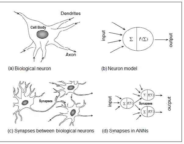
Figure 2.2: Neuron and its representation (Samarasinghe, 2006)
In ANNs, the neuron is the most fundamental element which makes up a neural pathway in its architecture. The neuron is also sometimes called as unit, node, perceptron or processing unit. It received input signals either from an external input or from some other units. In neuron model, input signals are received accumulated or summed (∑) and processed further [𝑓(∑)] to produce an output. As neurons are interconnected to each other, this output signal becomes an input signal to other neuron and transmitted from one neuron to another neuron through connection between them until the process is completed and a result is generated. Each connection between neurons has different synaptic strength or connection strengths (weights), which must undergo adaptation during the learning process where the neuron learns patterns from the information it received.
17
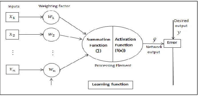
Figure 2.3: Computational elements in artificial neuron
Weighting factor: In ANNs, the neurons are connected by links and each
link has its own connection strength represented in numerical coefficient (Negnevitsky, 2005). These connections strengths are called synaptic weights and are the most important factor in determining the intensity of input signal received by neuron. They express the strength or the significance of each neuron input in the network. These weights can be adapted in response to various training sets and according to a network's specific topology or a learning rule (Sumathi and Paneerselvam, 2010). ANNs “learn” through repeated adjustment of these weights until the network reaches a steady state where there are no further significant changes in the synaptic weights.
Summation function: The initial step in the operation of processing units is
the summation of all weighted inputs. As showed as in Figure 2.3, the inputs and the corresponding weights are vectors that can be represented as (𝑥1, 𝑥2, . . . , 𝑥𝑛) and (𝑤1, 𝑤2, . . . , 𝑤𝑛). The input signals are the multiplication of each input with their corresponding weight which can be represented as 𝑤1𝑥1 = 𝑤1∗ 𝑥1, 𝑤2𝑥2 = 𝑤2 ∗ 𝑥2 and 𝑤𝑛𝑥𝑛 = 𝑤𝑛∗ 𝑥𝑛.The weighted input signals are summed to obtain a linear combination of the input signals 𝑤1𝑥1+ 𝑤2𝑥2+. . . +𝑤𝑛𝑥𝑛 before being processed further by the activation function.
Activation function: The result of the summation function is transformed to
18
is larger than the threshold value, the processing element generates a signal. If the sum of the input and weight products is lower than the threshold, no signal (or some inhibitory signal) is generated. The activation function employed for ANNs is generally non-linear. A nonlinear activation function limits the amplitude of the output neuron. Typically, activation functions have a “squashing” effect which prevents accelerating growth throughout the network (Cybenko, 1989; Sumathi and Paneerselvam, 2010).
Output function and error function: The output from the output function is
directly equivalent to the activation function's result. During the network training, the output for each training cycle is known as network output. In most learning networks, the difference between the network output and the desired output is calculated and denoted as the error. This error term is often called the network error. During neural learning, the network error is propagated backward to the previous layer. This back-propagated value, after being scaled by the learning function, is multiplied against each of the incoming connection weights to modify them before the next learning cycle.
Learning function: The purpose of the learning function is to modify or
update the variable connection weights on the inputs of each processing element according to some neural based algorithm. The process of updating these weights connections is also known as the adaption mode or training mode.
2.3.2 Different Models of Neural Networks
19
Generally, there are three types of ANNs architecture: feedforward neural networks, feedback neural networks, and self-organizing neural networks (Deb and Dixit, 2008). In feedforward network, the input signal travel through the network in forward direction, while in feedback network the outputs of some neurons are fed back to some neurons in layers before them, thus the input signal can travel both forward and backward directions. Self-organizing neural networks are distinct from the other two networks. It consists of neurons arranged in the form of a low dimensional grid where each input is connected related to all the output neurons. This type of network employs competitive learning method where each output neurons compete amongst themselves to be activated and the input signals are transmitted by the winning neurons. Among these architectures, the most common and widely used are the feedforward neural networks (Samarasinghe, 2006; Deb and Dixit, 2008; Sumathi and Paneerselvam, 2010).
2.3.3 Feedforward Neural Networks
The feedforward neural networks are the most well-known and commonly used models of ANNs (Epitropakis et al., 2006; Manohar and Reddy, 2008; Chen et al., 2013; Benzer and Benzer, 2015). The Feedforward neural networks structure is organized in a layered architecture, with each layer comprising one or more neurons. Each neuron is connected to one or more other neurons and the connections are only between consecutive layers, all in the same direction. All feedforward neural networks have input layer and output layer. Also, these networks can have numbers of layers and neurons per layer in between the input layer and output layer. These middle layers have no connection with the external world and hence are called hidden layers.
20
limited mapping ability and only capable of learning linearly separable patterns. On the other hand, multilayer perceptron had far greater processing power than the single layer perceptron and is capable of learning nonlinear decision surfaces.
2.3.4 Multilayer Perceptron
Multilayer layer perceptron (MLP) is a feedforward neural network which is formed by a collection of neurons that are connected by their associated weights in a hierarchical structure. The network is also known as first order neural network (Giles
et al., 1988). The MLP networks are capable of generating a complex mapping
between the input and the output and are capable of solving highly nonlinear problems (Cybenko, 1989). Minsky and Papert (1969) also stated that the MLP network is the most popular machine learning solution as it has the ability to build nonlinear decision surfaces in high dimensional problem space and is capable of providing more computational potential as compared to a single-layer perceptron network. Due to this capability, MLP has been successfully tested in many applications including the classification tasks (Murtagh, 1991; Widrow et al., 1994; Abu-Mahfouz, 2005; Bishop, 2006; Silva et al., 2008; Zabidi et al., 2010).
21
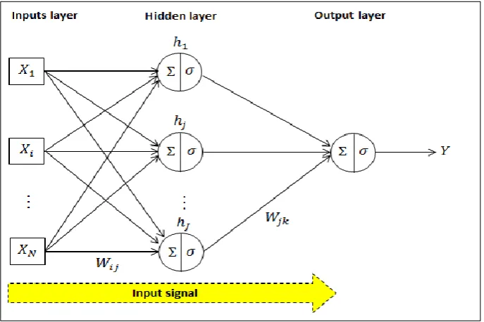
Figure 2.4: The basic structure of MLP
As shown in Figure 2.4, the MLP computes the network output, 𝑌 according to following equation:
𝑌 = 𝜎(∑ 𝑊𝑗𝑘𝜎(∑ 𝑊𝑖𝑗𝑋𝑖+ 𝑊𝑏𝑗) + 𝑊𝑏𝑘) 𝑁
𝑖=1 𝐽
𝑗=1
(2.1)
where 𝑋𝑖 denotes the input value, 𝑊𝑖𝑗 is the weights from the input layer to the
hidden layer, 𝑊𝑗𝑘 is the weights from the hidden layer to the output layer, 𝑊𝑏𝑗 is a
bias for hidden neuron, 𝜎 is a nonlinear activation function, and 𝑌 is the network output. The activation function 𝜎, acts as a squashing function that prevents accelerating growth throughout the network (Cybenko, 1989). The main activation
functions used in most MLP applications are the logistic sigmoid 𝜎 =1+𝑒1−𝑥 and
hyperbolic tangent 𝜎 = tanh (𝑥). These functions are mostly used because they are substantially outperforms the other activation functions, thus allowing the MLP to model well both strongly and slightly nonlinear mappings (Husaini et al., 2011).
22
expensive training algorithms and prone to get stuck in local minima. Another drawback of MLP is that the network needs a lot of training examples to be able to capture patterns in data which may affect the training process as this can lead to slow processing and unstable network behavior (Zaknich, 2003). Also, in order to achieve good classification ability, MLP requires a rather large amount of available measures such as fixing an appropriate number of neurons in each layer and determining a suitable number of hidden layers. As the number of hidden layers and nodes in MLP structure increases, the network architecture becomes more complex and training the network becomes more challenging. MLP networks with a large number of hidden layers and nodes also mean that they are having a large number of learning parameters. This will affect the MLP performance as the network with a large number of learning parameters tend to memorize the training data which may lead to over-fitting and poor generalization (Lawrence and Giles, 2000).
2.4 Higher Order Neural Networks
Higher-order Neural Networks (HONNs) expand standard feedforward neural networks structure by including enhanced nodes at the input layer that provide the network with a complete understanding of the input patterns and their relations (Epitropakis et al., 2006). The aim of HONNs is to replace the hidden neurons found in the first order neural network or commonly known as MLP to reduce the complexity of their structure (Giles and Maxwell, 1987). Therefore, HONNs distinguish themselves from ordinary feedforward networks by the presence of high order terms in the network. In ordinary feedforward networks architecture, neural inputs are combined using the summing operation only. However, in HONNs architecture, the network combines input of several neurons in another way than summation, usually combined with multiplication operation (Hoogerheide, 2006). The number of inputs that are combined in a non-linear way is the ‘order’ of the network.
23
1987; Pao and Takefuji, 1992). The high order terms employed in the network also facilitate in constructing a nonlinear mapping that provides better classification capability as compared to the first order neural network (Guler and Sahin, 1994).
In order to overcome the limitations of conventional ANNs, some researchers have turned their attention to HONNs models (Chang and Cheung, 1992; Yatsuki and Miyajima, 2000; Ming et al., 2002; Shuxiang and Ling, 2008; Fallahnezhad et al., 2011). This is due to its capability to simulate higher frequency, higher-order nonlinear data, and consequently, provide superior simulations compared to the ordinary feedforward networks (Kanaoka et al., 1992; Ming et al., 2002). Several applications that have gain advantage by using HONNs include; prediction (Ming et al., 2002; John et al., 2006; Ghazali, 2007; Husssain et al., 2009; Husaini et al., 2011), function approximation (Ghosh and Shin, 1995; Xu and Zhang, 2002) , classification and pattern recognition (Ghosh and Shin, 1995; Kosmatopoulos et al., 1995; Dehuri et al., 2008; Jia-Wei and Jun, 2009).
Even though most neural networks models share a common goal in performing input-output mapping, their ability in handling different type of problems are distinguished by the different type of network architecture. For some tasks, HONNs are needed as ordinary feedforward network like MLP cannot escape from the problems of local minima trapping especially when involving a highly complex nonlinear problem (Chen and Leung, 2004; Ghazali, 2007).
2.4.1 Properties of HONNs
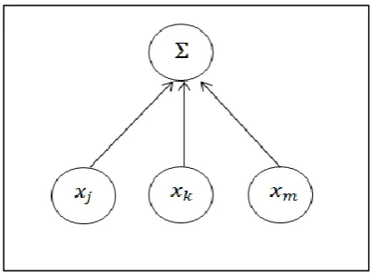
Most ordinary feedforward networks are first order neural networks. Neurons in ordinary feedforward network are also known as first-order neurons. First order neural networks models use a summation function ‘Σ’ which performs a linear
24
Figure 2.5: Inputs of neuron in first order neural network
The network is linear in the sense that they can capture only first-order correlations as they provide a linear summation of inputs (Giles and Maxwell, 1987). The non-linearity only occurs by means of application of a nonlinear (activation) function to the weighted sum of inputs in the neuron (Hoogerheide, 2006). They can be represented by:
𝑦𝑖(𝑥) = 𝜎 [∑ 𝑤𝑖𝑗𝑥𝑗 𝑁
𝑗
] (2.2)
where 𝑥 = {𝑥𝑗} is an input vector, 𝑤𝑖𝑗 is a weight parameters, N is the number of
elements in the input vector x, and 𝜎 is a sigmoid function (activation function). HONNs on the other hand, make use of multiplicative function or product term ‘П’ aside from the utilization of summation function ‘Σ’. According to Schmitt
(2002), the rationale of applying the multiplication operation in neural networks is to help to increase the computational power of the network. Schmitt (2002) also conveyed an empirical evidence on the existence of exponential and logarithmic dendritic processes in biological neural systems, in which support the application of multiplication and polynomial processing in artificial neural systems. Likewise, Durbin and Rumelhart (1990) also discussed on extending the standard MLP model with multiplicative or product units to increase the computational power in order to be able to work the same way as biological neural networks.
The HONNs’ architecture can be classified into three different groups based
REFERENCES
Abachizadeh, M., A. Yousefi-Koma and M. Shariatpanahi (2010). Optimization of a beam-type ipmc actuator using insects swarm intelligence methods. Proceedings of the ASME 10th biennial conference on engineering systems
design and analysis.
Abbas, H. M. (2009). "System Identification Using Optimally Designed Functional Link Networks via a Fast Orthogonal Search Technique." Journal of
Computers 4(2): 195-202.
Abdual-Salam, M. E., H. M. Abdul-Kader and W. F. Abdel-Wahed (2010). Comparative study between Differential Evolution and Particle Swarm Optimization algorithms in training of feed-forward neural network for stock price prediction. The 7th International Conference on Informatics and Systems (INFOS), 2010
Abedinia, O., N. Amjady and M. S. Naderi (2012). Multi-objective Environmental/Economic Dispatch using firefly technique. 11th International Conference on Environment and Electrical Engineering (EEEIC), 2012
Abu-Mahfouz, I.-A. (2005). "A comparative study of three artificial neural networks for the detection and classification of gear faults " International Journal of
General Systems 34(3): 261-277.
Aggarwal, C. C. (2014). Data classification: algorithms and applications, CRC Press.
Akay, B. and D. Karaboga (2010). "A modified Artificial Bee Colony algorithm for real-parameter optimization." Information Sciences In Press, Corrected Proof. Al-Jarrah, O. and A. Arafat (2015). "Network Intrusion Detection System Using Neural Network Classification of Attack Behavior." Journal of Advances in
Information Technology Vol 6(1).
Al-Shayea, Q. K. (2011). "Artificial neural networks in medical diagnosis."
150
Alweshah, M. (2014). "Firefly Algorithm with Artificial Neural Network for Time Series Problems." Research Journal of Applied Sciences, Engineering and
Technology 7(19): 3978-3982.
Amato, F., A. Lopez, E. M. Peña-Méndez, P. Vaňhara, A. Hampl and J. Havel (2013). "Artificial neural networks in medical diagnosis." Journal of applied
biomedicine 11(2): 47-58.
Anastassiou, G. A. (2011). "Multivariate sigmoidal neural network approximation."
Neural Networks 24(4): 378-386.
Artyomov, E. and O. Yadid-Pecht (2005). "Modified high-order neural network for invariant pattern recognition." Pattern Recognition Letters 26(6): 843-851. Azami, H., S. Sanei and K. Mohammadi (2011). "Improving the neural network
training for face recognition using adaptive learning rate, resilient back propagation and conjugate gradient algorithm." Journal of Computer
Applications 34(2): 22-26.
Bacanin, N. and M. Tuba (2014). "Firefly Algorithm for Cardinality Constrained Mean-Variance Portfolio Optimization Problem with Entropy Diversity Constraint." The Scientific World Journal 2014: 721521.
Banati, H. and M. Bajaj (2011). "Fire fly based feature selection approach." IJCSI
International Journal of Computer Science Issues 8(4).
Bandyopadhyay, S., S. K. Pal and B. Aruna (2004). "Multiobjective GAs, quantitative indices, and pattern classification." IEEE Transactions on
Systems, Man, and Cybernetics, Part B: Cybernetics 34(5): 2088-2099.
Basu, J. K., D. Bhattacharyya and T.-h. Kim (2010). "Use of artificial neural network in pattern recognition." International journal of software engineering and its
applications 4(2).
Benzer, R. and S. Benzer (2015). "Application of artificial neural network into the freshwater fish caught in Turkey." International Journal of Fisheries and
Aquatic Studies 2015 2(5): 341-346.
Bijami, E., M. Shahriari-kahkeshi and H. Zamzam (2011). Simultaneous coordinated tuning of power system stabilizers using artificial bee colony algorithm. 26th
international power system conference (PSC).
Bing, Y. and H. Xingshi (2006). Training radial basis function networks with differential evolution. 2006 IEEE International Conference on Granular
151
Bishop, C. M. (2006). Pattern Recognition and Machine Learning (Information
Science and Statistics), Springer-Verlag New York, Inc.
Blum, C. and X. Li (2008). Swarm Intelligence in Optimization. Swarm Intelligence. C. Blum and D. Merkle, Springer Berlin Heidelberg: 43-85.
Bonabeau, E., M. Dorigo and G. Theraulaz (1999). "Swarm Intelligence: From Natural to Artificial Systems." Oxford University Press, NY.
Borra, S. and A. Di Ciaccio (2010). "Measuring the prediction error. A comparison of cross-validation, bootstrap and covariance penalty methods."
Computational Statistics & Data Analysis 54(12): 2976-2989.
Bullinaria, J. and K. AlYahya (2014). Artificial Bee Colony Training of Neural Networks. Nature Inspired Cooperative Strategies for Optimization (NICSO
2013). G. Terrazas, F. E. B. Otero and A. D. Masegosa, Springer
International Publishing. 512: 191-201.
Ch, S. and S. Mathur (2012). "Particle swarm optimization trained neural network for aquifer parameter estimation." KSCE Journal of Civil Engineering 16(3): 298-307.
Chang, C. and J. Y. Cheung (1992). Backpropagation algorithm in higher order neural network. International Joint Conference on Neural Networks, 1992.
IJCNN.
Chen, A.-S. and M. T. Leung (2004). "Regression neural network for error correction in foreign exchange forecasting and trading." Computers & Operations
Research 31(7): 1049-1068.
Chen, C.-H., T.-K. Yao, C.-M. Kuo and C.-Y. Chen (2013). "RETRACTED: Evolutionary design of constructive multilayer feedforward neural network."
Journal of Vibration and Control 19(16): 2413-2420.
Chen, C., S. Duan, T. Cai and B. Liu (2011). "Online 24-h solar power forecasting based on weather type classification using artificial neural network." Solar
Energy 85(11): 2856-2870.
Chen, T. and R. Xiao (2014). "Enhancing Artificial Bee Colony Algorithm with Self-Adaptive Searching Strategy and Artificial Immune Network Operators for Global Optimization." The Scientific World Journal 2014: 12.
Cherkassky, V., J. H. Friedman and H. Wechsler (2012). From statistics to neural
networks: theory and pattern recognition applications, Springer Science &
152
Chi-Hsu, W. and H. Kun-Neng (2009). High-Order Hopfield-based neural network for nonlinear system identification. IEEE International Conference on Systems, Man and Cybernetics, 2009.
Chidambaram, C. and H. S. Lopes (2009). A new approach for template matching in digital images using an Artificial Bee Colony Algorithm. World Congress on
Nature & Biologically Inspired Computing, 2009. NaBIC 2009. .
Chien-Cheng, L., C. Pau-Choo and C. Yieng-Jair (2005). Classification of liver diseases from CT images using BP-CMAC neural network. 9th International Workshop on Cellular Neural Networks and Their Applications, 2005
Chien-Cheng, Y. and L. Bin-Da (2002). A backpropagation algorithm with adaptive learning rate and momentum coefficient. Proceedings of the 2002
International Joint Conference on Neural Networks, 2002. IJCNN '02. .
Cismondi, F., A. S. Fialho, S. M. Vieira, S. R. Reti, J. M. Sousa and S. N. Finkelstein (2013). "Missing data in medical databases: Impute, delete or classify?"
Artificial Intelligence in Medicine 58(1): 63-72.
Coello, C. A. C., G. T. Pulido and M. S. Lechuga (2004). "Handling multiple objectives with particle swarm optimization." IEEE Transactions on
Evolutionary Computation 8(3): 256-279.
Cortes, C. and V. Vapnik (1995). "Support-Vector Networks." Machine Learning 20(3): 273-297.
Cox, C. and R. Saeks (1998). Adaptive critic control and functional link neural networks. 1998 IEEE International Conference on Systems, Man, and
Cybernetics, 1998. .
Cuevas, E., F. Sención-Echauri, D. Zaldivar and M. Pérez-Cisneros (2012). "Multi-circle detection on images using artificial bee colony (ABC) optimization."
Soft Computing 16(2): 281-296.
Curram, S. P. and J. Mingers (1994). "Neural Networks, Decision Tree Induction and Discriminant Analysis: An Empirical Comparison." The Journal of the
Operational Research Society 45(4): 440-450.
Cybenko, G. (1989). "Approximation by superpositions of a sigmoidal function."
Math. Contr. Signals Syst 2: 303-314.
Dash, P. K., A. Liew and H. P. Satpathy (1999). "A functional-link-neural network for short-term electric load forecasting." Journal of Intelligent & Fuzzy