Simulation of Microbial Depolymerization Process with Exponential Consumption of Carbon Source

(1)

2016 International Conference on Computer, Mechatronics and Electronic Engineering (CMEE 2016) ISBN: 978-1-60595-406-6

Simulation of Microbial Depolymerization Process with Exponential

Consumption of Carbon Source

Masaji WATANABE

1,*

and Fusako KAWAI

2

1

Graduate School of Environmental and Life Science, Okayama University, Japan

2

Center for Fiber and Textile Science, Kyoto Institute of Technology, Japan *Corresponding author

Keywords: Biodegradation, Polymer, Mathematical model, Numerical simulation, Inverse problem.

Abstract. Mathematical techniques were applied to a microbial depolymerization process of exogenous type. Experimental results were incorporated into analysis, and a microbial depolymerization process of polyethylene glycol was simulated. Inverse problems for molecular factor and time factor of a degradation rate are described and numerical techniques are illustrated.

Introduction

Microbial depolymerization processes are classified into exogenous type and endogenous type. Molecules reduce in size through successive liberation of monomer units from their terminals in an exogenous type depolymerization process. Polyethylene (PE) is one of polymers that are depolymerized in exogenous type depolymerization processes. A depolymerization process of PE involves two primary factors, gradual weight reduction due to -oxidation, and direct consumption by cells. A PE molecule liberates a monomer unit (CH2CH2) in one cycle of -oxidation, and it undergoes successive -oxidation processes until it becomes small enough to be absorbed directly into cells. The scenario was modeled mathematically for simulation of PE biodegradation processes [1].

Polymers that are depolymerized in exogenous type depolymerization processes also include polyethylene glycol (PEG). Polyethers are polymers that are expressed by the structural formula HO(R-O)nH, and PEG is one of polyethers (R = CH2CH2). PEG is depolymerized liberating C2 compounds [2]. Mathematical techniques developed for PE biodegradation were applied to biodegradation of PEG [3]. Weight distributions with respect to the molecular weight before and after cultivation of microbial consortium E-1 was incorporated into inverse analysis of degradation rates, and initial value problems were solved numerically for simulation of PEG biodegradation processes. Time dependence of degradation rates was also taken into consideration for modeling and simulation of exogenous type depolymerization processes of PEG [4].

Molecules are broken up arbitrarily in endogenous type depolymerization processes. Polymers that are depolymerized in endogenous type depolymerization processes include polyvinyl alcohol (PVA) and polylactic acid (PLA). A mathematical model was proposed for an enzymatic depolymerization process of PVA [5], and it was applied to enzymatic hydrolysis of PLA. Degradabilities of PVA and PLA were compared [6]. Time dependence of the degradation rate was also incorporated into formulation of a PLA depolymerization process [7]. A model proposed for endogenous type depolymerization processes was reformulated for application to exogenous type depolymerization processes of PEG [8] and PE [9]. Mathematical techniques developed for the PE biodegradation [9] were applied to depolymerization processes of PEG [10]. Time dependence of degradability was incorporated into modeling of PEG depolymerization processes [10].

(2)

presented. Weight distributions of PEG before and after cultivation of microbial consortium E1 for one day, three days, five days, seven days, and nine days were introduced into analysis.

Formulation of Exogenous Type Microbial Depolymerization Process with Microbial Consumption of Carbon Source

Let w



t,M



[mg] be the weight distribution with respect to the molecular weight M and 

 

t be the microbial population at time t, such that the total weight of residual polymer v

 

t for AM B at time t is

 





B



,



.

Awt M dM t

v

(1) In particular, ｔhe total weight of residual polymer at time t, v

 

t is given by

 



,



.

0





 w t M dM t

v

(2) The total weight of residual polymer (2) is approximated with the integral (1) for appropriate values of

A and B.

The following system of equations (3), (4) was proposed in previous studies [13, 12, 11, 10].

 

_

 



  

,

 

,



_,

  



M _K K q M K wt K dK

M w

M t

t

w _ _ _

(3)

 





,

1  



   

 

   

t v h k dt d

(4) where

 





, log2.

1

,

L e

K e K

d Me

M

c _K

K

M 

 

   __ 

Here L is the molecular weight of monomer unit liberated from a molecule in one cycle of exogenous type depolymerization process, e.g. PE: L28 (CH₂CH₂), PEG: L44, (CH₂CH₂O ), and function 

 

M is the molecular factor of the degradation rate. Function 

 

t is the time factor of the degradation rate that corresponds to the microbial population. System of equations (3), (4) form an initial value problem with the initial condition



0,M



f₀

 

M ,

w 

(5)

 

0 ₀,

 

(6) where f₀

 

M and ₀ are the initial weight distribution and the initial microbial population, respectively.

Change of Variables and Inverse Analysis for Molecular Factor of Degradation Rate in Exogenous Type Depolymerization Process

Given the initial weight distribution f0

 

M and the initial microbial population, initial value problem

(3)

 

. 0



 t ds s   (7) Let W



,M

 

wt,M

        

, S  t, V  vt . The change of variables (7) converts the equations (3) and (4) to the equations (8) and (9), respectively

 



       



 , ,

   

M K d K W K dK

M c W M

W _ _ _

 ₍₈₎

 





. 1 _         



V h k d dS (9) suppose that F1

 

M and F2

 

M are weight distributions at  1 and  2, respectively, where

2 1

0  . When the molecular factor 

 

M is prescribed, equation (8) and the initial condition



M



F

 

M

W ₁,  ₁ ₍₁₀₎

form an initial value problem for W



,M



. Equation (8), the initial condition (10) and the additional condition



M



F

 

M

W ₂,  ₂ ₍₁₁₎

form an inverse problem for the molecular factor



 

M , for which the solution of the initial value problem (8), (10) also satisfies the condition (11). Numerical techniques to solve the inverse problem were developed in previous studies [15, 16]. Weight distributions after cultivation of the microbial consortium E-1 for one day and three days were assigned to the functions f1

 

M and f2 M ,

respectively, and ₁ 0 and 2 2 are set, and the inverse problem for the molecular factor 

 

M was solved numerically.

Inverse Analysis for Time Factor of Degradation Rate in Exogenous Type Depolymerization Process

Once the molecular factor 

 

M was found, the equation (8) is solved W



,M



with an appropriate initial condition



0,M



f0

 

M ,

W  ₍₁₀₎

where f₀ M is the initial weight distribution before cultivation. In a previous study,

 







3.2 4.2



10 , 10 , ,  





W M dM A B

V B

A 



was shown to be well approximated as an exponential function V

   

 V 0e. It was shown that

11859 . 0



 [11]. Here, 1 was set, that is, a further change variables from  to  was made. Let



 , R

 

 S

 

 , U

 

 V

 

 . Equation (4) leads to

Let , R

 

 , U

 

 , and h/ be denoted by



, S

 

 , V

 

 , and h, respectively, so that the equation (9) holds. Given weight distributions before and after cultivation of microbial consortium E1 for one

day, three days, five days, seven days, and nine days, correspondence between values of t and values

of  was obtained.

(4)

Note that the solution of the equation (9) with initial value ₀ is not only a function of



but also a function of ₀, k, and h, and denote it by S



,₀,k,h



. In view of the definition (7),

t

is expressed by tq



,₀,k,h



, where









.

, , , ,

, ,

0

0 





 



h k r S

dr h

k q

(12) Given three pairs of values of

t

and



,



t₁,₁



,



t₂,₂



, and



t₃,₃



such that t₁t₂t₃ and

3 2 1  

   , let



₀,k,h

 

q , ₀,k,h



t



i1,2,3



,

g_i  _i  _i

and consider the three equations for the three unknowns ₀, k, and h,



₀,k,h



0



i1, 2, 3



,

g_i  ₍₁₃₎

In a previous study, application of the Newton-Raphson method and the bisection method to the

system of equations (13) was demonstrated. For a fixed value of h, the Newton-Raphson method was

applied to the first two equations of the system (13) to generate functions 

 

h and 

 

h that satisfy

   



, ,



0, ₂



   

, ,



0.

1 h h h  g h h h 

g     ₍₁₄₎

Then the bisection method was applied to the equation

   



, ,



0 3 h h h 

g  

[image:4.595.67.526.488.646.2]

(15)

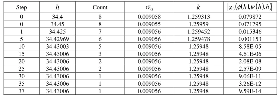
Table 1. Convergence of the Newton-Raphson method and the bisection method. The table shows that it took thirty seven steps of the bisection method for g₃





   

h, h,h



to reduce to the value less that 1012. Entries in the column “Count“ are the numbers of iterations for errors between two successive approximate solutions the system (14) to reduce to

the value less than 1012.

Step h Count ₀ k g₃





   

h, h,h



0 34.4 8 0.009058 1.259313 0.079872

0 34.45 8 0.009055 1.25959 0.071795

1 34.425 7 0.009056 1.259452 0.015346

5 34.42969 6 0.009056 1.259478 0.001153

10 34.43003 5 0.009056 1.25948 8.58E-05

15 34.43006 3 0.009056 1.25948 4.61E-06

20 34.43006 2 0.009056 1.25948 2.08E-08

25 34.43006 2 0.009056 1.25948 2.57E-09

30 34.43006 1 0.009056 1.25948 9.06E-11

35 34.43006 1 0.009056 1.25948 3.26E-12

(5)

[image:5.595.59.537.77.250.2]

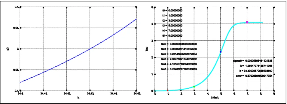
Figure 1. Graph of g₃





   

h, h,h



and the graph of



q



,₀,k,h



,



.

Summary

Equations (4) and (9) were proposed in a previous study. Weight distributions before and after microbial consortium E1 for two days, four day and seven days were introduced into analysis. The Newton-Raphson method was applied to the system of equations (13) under the assumption

   

_ _ 

e V

V 0 where  was obtained from a numerical solution of the initial value problem (8), (10). In this study, the application of the Newton-Raphson method and the bisection method to the system of equations (13) was demonstrated for 1. Once appropriate values of the parameters ₀, k, and

h were found, 

 

t is given by 

   

t S / , t q



,₀,k,h



, and the transition of weight distribution was simulated by solving the initial value problem (3), (5). Experimental data may be available in terms of residual polymer given at discrete points of time. Our techniques have potential applicability to such a case.

Acknowledgement

The authors thank Ms. Y. Shimizu for her technical support. This work was supported by JSPS KAKENHI Grant Number 24540127.

References

[1] Masaji Watanabe, Fusako Kawai, Masaru Shibata, Shigeo Yokoyama, Yasuhiro Sudate, Shizue Hayashi, Analytical and computational techniques for exogenous depolymerization of xenobiotic polymers, Mathematical Biosciences 192 (2004) 19-37.

[2] Fusako Kawai, Takuhei Kimura, Masahiro Fukaya, Yoshiki Tani, Koichi Ogata, Tamio Ueno, Hiroshi Fukami, Bacterial oxidation of polyethylene glycol, Applied and Environmental Microbiology, Vol. 35, No. 4, 679-684, 1978.

[3] M. Watanabe, F. Kawai, Numerical simulation of microbial depolymerization process of exogenous type, Proc. of 12th Computational Techniques and Applications Conference, CTAC-2004, Melbourne, Australia in September 2004, Editors: Rob May and A. J. Roberts,

ANZIAM J. 46(E) pp.C1188-C1204, 2005.

http://journal.austms.org.au/ojs/index.php/ANZIAMJ/article/view/1014

[4] M. Watanabe and F. Kawai, Effects of microbial population in degradation process of xenobiotic polymers, In P. Howlett, M. Nelson, and A. J. Roberts, editors, Proceedings of the 9th Biennial Engineering Mathematics and Applications Conference, EMAC-2009, volume 51 of ANZIAM J.,

pages C682-C696, September 2010.

(6)

[5] Masaji Watanabe, Fusako Kawai, Mathematical modelling and computational analysis of enzymatic degradation of xenobiotic polymers, Applied Mathematical Modelling 30 (2006) 1497-1514.

[6] Masaji Watanabe, Fusako Kawai, Sadao Tsuboi, Shogo Nakatsu, Hitomi Ohara, Study on Enzymatic Hydrolysis of Polylactic Acid by Endogenous Depolymerization Model, Macromolecular Theory and Simulations 16 (2007) 619-626.

[7] M. Watanabe, F. Kawai, Modeling and analysis of biodegradation of xenobiotic polymers based on experimental results, Proceedings of the 8th Biennial Engineering Mathematics and Applications Conference, EMAC-2007, Editors: G. N. Mercer and A. J. Roberts, ANZIAM J. 49

(EMAC-2007) pp.C457--C474, March 2008.

[8] M. Watanabe and F. Kawai, Study of biodegradation of xenobiotic polymers with change of microbial population, In W. McLean and A. J. Roberts, editors, Proceedings of the 15th Biennial Computational Techniques and Applications Conference, CTAC-2010, volume 52 of ANZIAM

J., ages C410-C429, July 2011.

[9] Watanabe M, Kawai F (2012) Modeling Biodegradation of Polyethylene with Memoryless Behavior of Metabolic Consumption, J Bioremed Biodegrad 3: 146.

[10] M. Watanabe and F. Kawai, Study on microbial depolymerization processes of xenobiotic polymers with mathematical modelling and numerical simulation, In Mark Nelson, Mary Coupland, Harvinder Sidhu, Tara Hamilton, and A. J. Roberts, editors, Proceedings of the 10th Biennial Engineering Mathematics and Applications Conference, EMAC-2011, volume 53 of

ANZIAM J., pages C203-C217, June 2012.

[11] Masaji Watanabe, Fusako Kawai, Numerical Techniques for Inverse Problems from Modeling of Microbial Depolymerization Processes, International Journal of Applied Engineering Research ISSN 0973-4562 Volume 11, Number 8 (2016) pp 5461-5468.