Effects of Geometry on Speed–Flow Relationships for Two–Lane Single Carriageway Road

2016 International Conference on Computational Modeling, Simulation and Applied Mathematics (CMSAM 2016) ISBN: 978-1-60595-385-4

Effects of Geometry on Speed–Flow Relationships for Two–Lane Single

Carriageway Roads

Othman CHE PUAN

and Nur Syahriza MUHAMAD NOR

*Corresponding author

Keywords: Speed-Flow relationship, Capacity, Two-lane single carriageway road.

Abstract. Speed–flow relationship is usually used as a basis for the performance and capacity analysis of a highway segment. This paper presents the preliminary result of a study carried out to evaluate the effects of road geometry on speed–flow relationship for two–lane single carriageway roads. Speed and traffic volume data at five uninterrupted two–lane single carriageway road segments located in different parts of Malaysia were collected using an automatic traffic counter equipment. Result of the analysis shows that speed and traffic flow variables for a single carriageway road were linearly related. The percentage of no passing zone, road bendiness and hilliness, and the presence of minor junctions were found to have negative effects on the speed–flow curve. The speed–flow–geometry relationship developed in the study produces the estimates of travel speed higher than the values estimated using both USHCM and British models and lower than the MHCM’s model. However, more data representing large range of traffic conditions and roadway characteristics are required to enhance the accuracy of the speed–flow–geometry relationship developed in the study.

Introduction

Highway capacity is generally defined as “the maximum number of vehicles that can pass a given point during a specified period under prevailing roadway, traffic, and control condition” [1]. Theoretically, highway capacity is often derived from speed–flow–density relationships [2]. American Transportation Research Board (TRB) [3] suggested that capacity analysis is to be conducted for segments of a facility having uniform traffic, roadway, and control conditions. In practice, the overall level of service of a facility is based on the road segment with the poorest operating conditions.

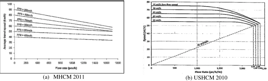
Many reports, for instance as reported by Garber and Hoel [4] and Heydecker and Addision [5], indicate that the speed–flow–density relationships are in a parabolic form. However, the TRB’s speed–flow curve [1, 3] does not seem to fit the parabolic–formed of relationship. The speed–flow model developed for the Malaysian Highway Capacity Manual (MHCM 2011), on the other hand, is a linear–formed of relationship as shown in Fig. 1(a) [6]. The recent USHCM’s speed–flow relationship is also shown in Fig. 1(b) for comparison.

(a) MHCM 2011 (b) USHCM 2010

It is interesting to note that the linear–formed of the speed–flow relationship suggested by the MHCM 2011 appears to support the findings of three major studies carried out in Great Britain in early 1970, 1980 and 1990, i.e. by Duncan [7], Transport and Road Research Laboratory [8, 9] and Lee and Brocklebank [10]. The speed–flow relationships developed by Lee and Brocklebank [10], which was adopted in the British Department of Transport’s economic assessment of road schemes software (COBA) [11], take account explicitly the effects of almost every aspects of road geometry including visibility and junctions.

This paper discusses the effects of road geometry on speed–flow relationships for Malaysian road traffic conditions.

Methodology

Site Selection

The survey sites were selected based on the following criteria [10, 12], i.e. (a) road segment is relatively homogeneous in geometric characteristics, (b) there is no major junction within the segment or within at least 1km of its endpoints, (c) there is no road works along the segment, and (d) the length of the road segment is more than 2 km.

The selection criteria defined above were adopted to ensure that there is no interruption on the speed behaviour and the motorist’s selected speed is in a stable condition. In this study, five uninterrupted two–lane single carriageway road segments were considered. The characteristics of the road segments considered in the study are tabulated in Table 1. The definitions of hilliness and bendiness are illustrated in Fig. 2. The average bendiness and average hilliness were calculated using Eq. 1 and Eq. 2.

Table 1. Site characteristics. Site

no. Site ID

Length (m) Both lane width (m)

Shoulder (m) Verge (m) Hilliness (m/km)

Bendiness (°/km)

AB BA AB BA

1. J/J46/1A 5,060 7.00 1.00 1.00 3.00 3.00 20.93 71.34

2. C/FT003/1A 2,390 7.00 2.50 2.50 6.00 4.50 10.13 10.46

3. J/FT003/1A 2,600 7.30 0.70 0.70 4.00 4.50 19.31 19.81

4. P/P145/1A 4,250 7.00 0.15 0.00 3.00 2.50 22.07 26.35

5. S/SA2/1B 5,380 6.50 0.00 0.00 1.60 2.60 30.67 48.51

(a) Plan view (b) Longitudinal profile Figure 2. (a) Plan View Bendiness and (b) Hilliness.

Average bendiness, °/km = (θ_{1 +} θ_{2 +} θ_{3 + …….. +} θ_{n) / Length (1)}

Average hilliness, m/km = (h1 + h2 + h3 + ……… + hn) / Length (2)

Data Collection and Analysis Method

The speed and flow data was collected using an automatic traffic counter (ATC). An ATC was used

because it allows traffic data to be collected for a long period of time.

the 15–minute traffic volume by 4 as suggested by TRB [1]. The average spot speeds or time-mean speeds were then converted to space mean speed using Eq. 3 [6, 12].

us = 1.016ut – 1.704 (3)

where us is space mean speed while ut is time mean speed.

Results and Discussion

Speed–Flow Relationship

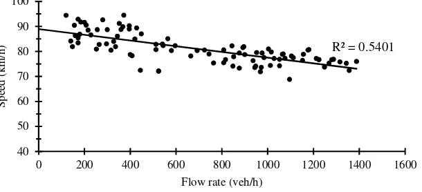
Ninety six sets speed–flow data were collected for each of the sites considered in the study. Fig. 3 shows the variations of speed–flow data for one of the road segments evaluated in the study. It can be seen that a negative linear form of relationship with a reasonable degree of correlation can be developed for the road segment. Such a speed–flow trend is consistent with the general understanding that speed decreases as traffic volume increases. The speed at which the trend line intercepts the

vertical axis is normally referred to as the free–flow speed, Uf, for the road segment considered. The

free–flow speeds derived from this study were found to be consistent with the speed limits posted for the corresponding road segments.

Figure 3. Scatter plot of speed–flow data for Site C/FT003/1A.

Effects of Geometry on Speed–Flow Relationship

A regression analysis was performed to evaluate the effects of various aspects of road geometry on speed–flow relationship. The aspects considered in the analysis are the total width of the carriageway in meter (CWID), shoulder width in meter (SWID), verge width in meter (VERGE), % no passing zone (NPZ), bendiness in degree/km (BEND), hilliness in m/km (HILL), number of minor left (LJUNCT) and right junction (RJUNCT) per km, opposing flow in veh/h (OPFLOW) and proportion of heavy vehicles (PHV).

Analysis indicates that the CWID, SWID, VERGE, OPFLOW and PHV have no significant effect on the average speed of vehicles. This is probably because the variations in the width of the traffic lane, shoulder and verge of road segments considered in the study are not that significant. The insignificant influence of opposing flow on speed, on the other hand, is probably due to high percentage of non-overtaking sections along the roadways. The small amount of heavy good vehicles in the traffic streams, i.e. 1.8% to 5.1%, did not affect the overall travel speed of traffic. Therefore, these variables were excluded from the relationship. Finally, speed–flow–geometry relationship developed is as shown in Eq. 4.

U = 128.01 – 0.02016 x Q – 0.05442 x NPZ – 0.2436 x BEND – 0.02739 x HILL

– 7.73957 x LJUNCT – 11.6994 x RJUNCT (4)

where U and Q are speed and flow, respectively. All other variables are as defined earlier. R² = 0.5401

40 50 60 70 80 90 100

0 200 400 600 800 1000 1200 1400 1600

S

p

ee

d

(

k

m

/h

)

The R2–value for the relationship is 0.77, i.e. a value indicating a reasonably good relationship exists between speed and the various influencing factors considered in the analysis. The signs associated with each of the variables in Eq. 4 are consistent with what would be expected intuitively. The constant in Eq. 4 can be interpreted as free flow speed and may be described as the mean desired speed. However, here constant includes road geometry related modifying factors and, the definition of desired speed needs to be re-considered. Desired speed may be defined as a driver’s desired speed on a level straight road in the absence of any impeding vehicles. This definition applies to the constants in Eq. 4. The actual driver’s desired speed can be taken as the basic desired speed modified by road geometry. This is obtained by an appropriate combination of the constant and road geometry related terms in the relationships such as found in Eq. 4.

To visualise a typical form of the speed–flow curve for a specified single carriageway section, the relationship given by Eq. 4 is plotted in Fig. 4. The speed–flow curves based on USHCM 2010 [1], MHCM 2011 [6] and Lee and Brocklebank [10] were also plotted for a comparison. The plots are based on the characteristics of road segment marked as J/J46/1A given in Table 2.

It can be seen from Fig. 4 that for a given traffic volume under stable flow conditions, both USHCM 2010 and British’s speed–flow curves predicted a much lower travel speeds compared with both the observed data and the model developed in this study. The observed data in general is scattered around the proposed model.

Figure 4. Comparisons of Speed–Flow Curves for Site J/J46/1A.

Table 2. Parameter for Site J/J46/1A.

Parameter Value

Lane Width, Shoulder, Verge 7.0m, 1.0m, 3.0m

No Passing Zone 52.5%

Bendiness, Hilliness 71.34 degree/km, 20.93 m/km

No of Minor Left & Right Junctions 1.38/km, 1.38/km

Proportion Heavy Vehicle 0.022

The MHCM 2011’s speed–flow relationship, on the other hand, predicts the estimates of travel speed which are relatively higher than the observed values and other models as can be seen in Fig. 4.

Summary

This paper discusses the relationship between speed, flow and geometry for a two–lane single carriageway road based on a range of traffic flow and geometry conditions. The main findings of the study can be summarized as follows:

• A parabolic curve describing speed–flow relationship, as it is traditionally understood, is

difficult to be developed because traffic flow breakdowns seldom occur under uninterrupted flow 40

50 60 70 80 90

0 100 200 300 400 500 600 700 800

A

v

er

ag

e

T

ra

v

el

S

p

ee

d

,

k

m

/h

Flow, veh/h/direction Observed data

conditions. In fact, there is no published information about traffic operations in congested situations on, or at capacity of, single carriageway roads in Malaysia;

• Under stable flow conditions, the average speed of vehicles on a single carriageway road

appear to be linearly related with traffic flow;

• No passing zone, the presence of minor junctions, bendiness and hilliness reduced the average

speed of vehicles and hence affect the speed–flow curve for a single carriageway road; and

• Applicability of USHCM and existing MHCM to the analysis of speed–flow relationships and

hence the capacity of single carriageway roads for Malaysian traffic conditions need further verifications.

Acknowledgement

This research was financially supported by the Ministry of Higher Education Malaysia and Universiti Teknologi Malaysia (FRGS/2/2014/TK07/UTM/02/2-Q.J130000.7808.4F636). Special thanks to the Public Work Department Malaysia for the cooperation during data collection exercises.

References

[1] Transportation Research Board, Highway Capacity Manual. TRB, Washington, D.C. (2010)

[2] Minderhoud, M. M., Botma, H. and Bovy, P. H. L., Assessment of Roadway Capacity Estimation

Methods. In TRR: Journal of the Transportation Research Board. No. 1572. Transportation Research

Board, National Research Council, Washington D.C. (1997) 59-67.

[3] Transportation Research Board, Highway Capacity Manual. TRB, Washington, D.C. (2000)

[4] Garber N.J. and Hoel L.A., Traffic and Highway Engineering. 3rd ed. USA. (2001)

[5] Heydecker, B.G. and Addision, J.D., Analysis and Modelling of Traffic Flow under Variable

Speed limits. Transportation Research Part C. 19: (2011) 206-217.

[6] Highway Planning Unit, Malaysian Highway Capacity 2011, Ministry of Work, Malaysia.

(2011)

[7] Duncan, N.C., Rural Speed/Flow Relations. TRRL, Laboratory Report 651, Transport and Road

Research Laboratory, Crowthorne, U.K. (1974)

[8] Transport and Road Research Laboratory, A Study of Speed/flow/geometry relations on rural

single carriageways. TRRL LF923, Crowthorne, U.K. (1980a)

[9] Transport and Road Research Laboratory, Speed/flow/geometry formulae for rural single

carriageways. TRRL LF924, Crowthorne, U.K. (1980b)

[10] Lee, B.H. and Brocklebank, P.J., Speed-flow-geometry relationships for rural single

carriageway roads. TRRL Contractor Report 319, Transport and Road Research Laboratory, Crowthorne, U.K. (1993)

[11] Department of Transport, Design Manual for Roads and Bridges, Vol. 13, Economic Assessment of Road Schemes, HMSO, London, U.K. (1996)

[12] Leong, L.V. and Awang, M.A., Estimating Space-Mean Speed for Rural and Suburban

Highways in Malaysia. Journal of the Eastern Asia Society for Transportation Studies, Vol 9,