Multi platform Genomic Data Analysis Using Multimodal Autoencoder

2015 3rd AASRI Conference on Computational Intelligence and Bioinformatics (CIB 2015) ISBN: 978-1-60595-308-3

Multi-platform Genomic Data Analysis Using Multimodal Autoencoder

Hao Chen, Jiayuan Shi

College of Computer Science, Sichuan University, Chengdu, P. R. China

ABSTRACT: Analyzing genomic expression profile is a significant way to identify cancer subtypes which can reveal insightful information of cancer pathogenesis and thus improve the prediction of patients’ survival time. Many approaches have been developed to analyze the genomic data of different cancer subtypes; most of them, however, are only capable of analyzing the genomic data from a single platform, e.g., gene expression, miRNA expression, or DNA methylation. In this paper, we propose an unsupervised deep learning method based on the multimodal autoencoder (MMAE) that is capable of analyzing the cross-platform genomic data for cancer subtype identification. The method starts with applying entropy information to the ultra-high-dimensional genomic data to select genomic variables with good classification capabilities. The MMAE networks are then introduced to extract and fuse the features from different genomic platforms. The MMAE networks are thus capable of capturing both the intra-structures of genomic data from a single platform and the inter-correlations among different platforms. Finally, the K-means method is performed to cluster the patients into subtypes. Experiments on the ovarian (OV) cancer patient dataset show that the proposed method effectively extracts the latent features of the genetic data and successfully clusters the patients into different subtypes with distinct survival characters.

1 INTRODUCTION

Identification of cancer subtypes can reveal insightful information about cancer pathogenic mechanisms and thus provides useful information to guide the clinical therapy. The pathogenesis of cancer tumors is generally caused by different genetic mutations. Exploring the discrepancies of patients’ genetic expression features therefore plays a significant role in identifying cancer subtypes. It has been found that genetic expression features are highly correlated with clinical performance of patients, such as survival time and recurrence time. For example, [1] shows that the breast cancer patients who have good genetic expression profiles are more likely to live longer than those who have poor genetic expression profiles. Recently, high-throughput sequencing technologies rapidly accumulate large amounts of cross-platform genomic profiles of tumors, such as gene expression (GE), miRNA expression (ME) and DNA methylation (DM). A typical example is the Cancer Genome Atlas (TCGA) project, which has collected a large amount of cross-platform genomic data for exploring human cancers.

The large-scale cross-platform genetic data of tumors contain plentiful information about genetic expression characters, as well as provide the opportunities to discover the correlation among the genomic data from different platforms. Since the

method effectively extracts the latent features of the genetic data and successfully clusters the patient into different subtypes with distinct survival characters.

The rest of this paper is organized as follows. Section 2 presents the proposed method in details. Specifically, Section 2.1 introduces the entropy information to choose key genetic variables with good classification capability. Section 2.2 first presents the single autoencoder method, Section 2.3 then proposes the multimodal autoencoder (MMAE) networks, Section 2.4 finally describes the learning process of the MMAE networks. Section 3 shows experiment results on the OV cancer dataset from TCGA project with comparison of the K-means method. Analysis on the survival time with respect to the different cancer subtypes are also made in this section. Finally, Section 4 concludes this paper.

2 METHODS

2.1 Entropy Information

Entropy information is defined as the expected value of the information that is gathered from different sources. It characterizes the uncertainty about the source of information. The entropy information was firstly proposed by C E Shannon [7] and has been widely used in many applications [8], [9]. In the theory of entropy information, the smaller the occurrence probability of the information is, the greater amount of information it brings, and vice versa. Motivated by this property of the entropy information, we introduce a method to select important genetic data variables based on the amount of information they carry. The purpose of this step is to mine important genetic variables among the high-dimensional genetic data and then reduce the dimension of the original data vectors.

In cancer data analysis problem, we call the genomic data from each platform, e.g., gene expression (GE), miRNA expression (ME) and DNA methylation (DM), the genomic profile for each patient. Let X be a genetic variable of a platform’s genomic profile whose probability distribution is defined as

(1) s. t.

Where pi means the occurrence probability of the genomic variable X with value xi. The amount of information this genetic variable carries is defined as:

(2) The H value is calculated respectively for each genetic variable of each platform. Due to the property of the entropy information, the genetic variables with bigger H value carry more

information than the genetic variables with the smaller H value. Those variables thus present the good classification capability. We therefore choose those genetic variables with bigger H value and use them in the following steps.

2.2 Autoencoder

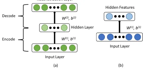
The autoencoder neural network [10], [11], [12] is an unsupervised learning method that consists of three layers: the input layer, the hidden layer, and the reconstruction layer. The goal of the autoencoder neural network is to learn an identity function that the output of the reconstruction layer approximates the input of the input layer. We use this network to learn a compressed representation and structure of the input genetic data. For a certain platform’s genetic profile, we set n be the total number of cancer patients, and set m be the total number of genomic variables for each patient. In this paper, our single modality autoencoder is a three layered neural network as shown in Figure 1(a). It consists of a layer of input neurons vi, i = 1, ..., m, a layer of hidden neurons hj, j = 1, ..., g, and a layer of output neurons rk, k = 1, ..., m. The number of input visible neurons is equal to the number of genomic profiles of each patient. Each connection between input and hidden neurons is associated with a specific weight. Let W(1) = (W(1)ji)g*m be the matrix representing the weights between the input layer and the hidden layer, where each element W(1)ji represents the weight of the corresponding connection between input neutron vi and hidden neutron hj; likewise, let W(2) be an m*g dimensional matrix representing the weights between the hidden layer and the reconstruction layers. Let b(1) = (b(1)1, ...,b(1)g) and b(2) = (b(2)1, ...,b(2)m) be the bias vectors of the input layer and the hidden layer, respectively. Since the reconstruction layer approximates the input layer through the hidden layer, the hidden layer could be treated as a low dimensional representation of the input genetic profiles as shown in Figure 1(b). Please note that autoencoders can be stacked upon each other to form a deep network, stacked autoencoder (SAE).

Figure 1. Structure of three layered autoencoder network and the learned features of this three layered autoencoder network.

W(1)_,b(1)

W(2)_,b(2)

ReconstructionLayer

InputLayer

(a)

HiddenLayer

Decode

Encode

W(1)_,b(1)

InputLayer

(b)

2.3 Multimodal Autoencoder

Recent work on deep learning [10] has examined how deep autoencoder networks can be trained to produce useful representations for image and text. We use an extension of autoencoder network with multi-platform input, which has been shown to learn meaningful features across audio and video modalities [4]. In our proposed method, autoencoder network acts as a layer-wise building block for our models.

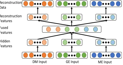
Figure 2. An example of a multimodal antuencoder (MMAE) model which takes DM, GE and ME respectively as input data.

Multi-platform genomic data, e.g., gene expression (GE), miRNA expression (ME) and DNA methylation (DM), universally have distinct statistical properties. To discover both the intra-structures and inter-correlations in different genomic platforms, we propose to apply deep learning framework, the multimodal autoencoder (MMAE), on the cross-platform genomic data. Figure 2 describes structure of the MMAE. A MMAE is a network of stacked autoencoders (SAE). At the bottom level, it contains separate SAE for each genomic platform, taking the raw genomic data as input. This allows the MMAE to learn useful features for each platform before they are combined as well as makes it easier for the model to learn higher-order correlations across different genomic platforms. Then the features of single platform will be combined together and fed into a joint autoencoder layer at the higher level, and the fused representation, which represents the common features across different genomic platforms, is learned. As shown in Figure 2, the input data involves three platforms – DM, GE and ME. Each set of hidden neurons outputs a low dimensional representation as modality-specific features of an individual genetic platform. Those modality-specific features are then combined together as the input of next joint autoencoder layer. The joint layer fuses the modality-specific features as the common features of cross-platform genetic data.

In our MMAE model, the hidden variables of single modality learned the intra-structures within each input genomic platform, while the joint layer hidden variables fuse these intra-structures for single platform and form a common representation of

inter-correlations among different platforms. It has been proved that MMAE can learn correlations across different modalities [4]. In the cross modality learning setting where audio and video are present during feature learning period, the deep MMAE is trained to reconstruct both modalities when given only video modality and thus discovers correlations across audio and video modalities.

2.4 Learning

For MMAE networks, we use backward propagation algorithm to train parameters of the network [13]. Specifically, the cost function for a single input sample is given by

2 ,

1

( , ; , ) ( )

2 W b

J W b x y = h x −y

(3) Where y is the input data, is the reconstructed input. The overall cost function is given by

1

2 ( )

1 ,

1 ( ) 2

1 1 1

1 1

( , ) ( )

2

( )

2

l l l

m i i

i W b

n S S l

l i j ji

J W b h x y

m

W

λ

+ =

−

= = =

  

= _{ } − _

 

 

+

∑

∑

∑ ∑

(4) Where m represents the number of patient samples. In Eq. 4, the first term is an average sum-of-squares error term, and the second term is a regularization term.

For each iteration, the parameters W and b are updated as follows

( ) ( )

( ) ( , )

l l

ij ij l

ij

W W J W b

W

α ∂

= −

∂ (5)

( ) ( )

( ) ( , )

l l

i i l

i

b b J W b

b

α ∂

= −

∂ (6) Where α _{is the learning rate.}

3 EXPERIMENTS AND ANALISIS

3.1 Sources of Data

We validate our proposed data analysis method on the ovarian (OV) cancer dataset from the TCGA. This dataset contains genetic data across 379 patients from different platforms, i.e., gene expression (GE), DNA methylation (DM) and miRNA expression (ME).

3.2 Experiment Details

The genetic data of OV cancer from all three platforms, gene expression (GE), miRNA expression (ME), and DNA methylation (DM), are taken in our experiments. As explained in Section 2, we firstly apply the entropy information method to find out the genetic variables with good classification capability in terms of the H value defined in Eq. 2. The H

Reconstruction Features

DMInput Fused

Features

GEInput MEInput Hidden

values are computed for GE data, ME data, and DM data, respectively. In our experiments, we choose 2000 GE variables, 500 ME variables and 2000 DM variables with bigger H values, respectively. Those selected variables will be used in the following steps.

We then apply the MMAE to those selected variables. As indicated in Figure 2, the single autoencoder model for each genetic platform is first established. For both the GE and the DM platform, we stack up two hidden layers, one with 400 neurons and another one with 100 neurons. For the ME platform, we use only hidden layer with 100 neurons. After extracting the features of each single platform, we use a joint autoencoder layer to fuse those features derived from all three platforms. The joint autoencoder contains one hidden layer with 40 hidden neurons. For each hidden neurons and output neurons, we use the sigmoid function [14] as the activation function. We add sparsity penalty term [13] to the cost function and set the sparsity parameter as 0.05. Finally, we apply K-means method to this feature space derived by the MMAE and cluster the 379 OV cancer patients into eight subtypes.

To guarantee that our proposed model learned the inter-correlations among different platforms, we use reconstruction error to evaluate what features that MMAE learned. Inspired by [4], we reconstruct modality-specific features from one platform using features from two other platforms and compare the reconstruction with original features. In practice, we set zero values for GE input features and original input values for the DM and ME features, but still require the network to reconstruct features from all the three platforms. To evaluate the reconstruction error, we set threshold value as 0.1 for output neurons due to the sparsity character of the output. We regard output neurons whose values are greater than 0.1 as activated and output neurons whose values are less than 0.1 as deactivated. The result shows that 71.1% output neurons for GE features which are activated with original GE input values are still activated when setting zero values for GE input features, which proves that our trained model learned inter-correlations among different platforms. 3.3 Analysis of Ovarian Cancer Patients

Table 1 shows the populations of eight subtypes. It is observed that those eight subtypes present biased population distribution. The subtype #5 has significant large population than the other subtypes.

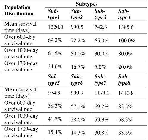
To investigate the survival characters of cancer patients in different subtypes, we use the clinical data from TCGA, which contains the survival time information for all 379 patients. Table 2 presents the mean survival time and the distribution of the survival rate over different survival time for different subtypes. As indicated in Table 2, more

than 80% patients in subtype #8 survive over 600 days. In comparison, only 65% patients in subtype #3 survive over 600 days. For 1000-day survival rate, subtype #1, #7, and #8 have more than 50% survival rate; by contrast, the subtype #3 and #6 only have up to 30% survival rate. Furthermore, more than 30% patients in subtype #1, #7 and #8 survive over 1700 days. However, this rate reduces to 5% for subtype #3. The above analysis might indicate that the symptoms of patients in subtype #1, #7 and #8 are mild whereas the symptoms of patients in subtype #3 and #6 are severe.

Table 1. Population distribution of eight subtypes.

Table 2. Survival time analysis of eight subtypes.

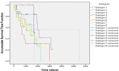
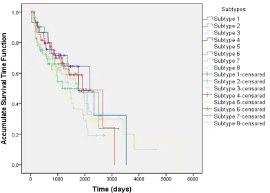
To validate our clustering results, we use the Kaplan-Meier plots to estimate the accumulate survival time function based on the survival time data. The results are shown in Figure 3. Figure 3 reveals that the survival functions of those eight subtypes are distinct from each other. Specifically, Figure 3 shows that patients in subtype #1 have higher probability to survive than those in subtype #3 and #6. Figure 4 further shows the estimated accumulate survival time function for subtypes #1, #3 and #6, respectively. The differences of survival time functions among those three subtypes are significant. The average 1000-day survival rate in subtype #1 is over two times higher than subtype #6, and at least 30% higher than subtype #3. This survival rate analysis indicates the feasibility of our proposed clustering schema.

Population Distribution

Subtypes

Subtype1 Subype2 Subype3 Subtype4

Population 26 18 20 5

Subtype5 Subtype6 Subtype7 Subtype8

Population 259 14 13 24

Population Distribution

Subtypes

Sub-type1

Sub- type2

Sub-type3

Sub- type4

Mean survival

time (days) 1220.0 990.5 742.3 1385.6

Over 600-day

survival rate 69.2% 72.2% 65.0% 100.0%

Over 1000-day

survival rate 61.5% 50.0% 30.0% 80.0%

Over 1700-day

survival rate 34.6% 16.7% 5.0% 20.0%

Sub-type5

Sub-type6

Sub-type7

Sub- type8

Mean survival

time (days) 974.9 990.9 1171.2 1410.8

Over 600-day

survival rate 58.3% 57.1% 69.2% 83.3%

Over 1000-day

survival rate 41.7% 28.6% 53.9% 58.3%

Over 1700-day

Figure 3. Accumulate survival time functions for eight subtypes clustered by MMAE method shown as Kaplan-Meier plots.

Figure 4. Accumulate survival time functionssss for three subtypes clustered by MMAE method shown as Kaplan-Meier plots.

To further evaluate our methods, we examine the expression of miRNA marker, miR-29. It had been found that expression levels of miR-29 family are associated with prognosis. The patients with significant down-regulated miR-29 had short survival time compared with those who presented relatively high levels of miR-29 [15]. We use the Z-score [16], the common method in gene analysis, to examine the miR-29a expression level of different subtypes. According to the survival time analysis in Table 2, we observed that patients in subtype #1, which has the highest miR-29a expression (Z-score=1.29), live 64.4% longer in average than patients in subtype #3, which has the lowest miR-29a expression (Z-score=-0.99). This observation is consistent with the analysis of MCL patients in [15]. In addition, one of the significant genes between subtypes is human Telomerase Reverse Transcriptase (hTERT). The hTERT is crucial for cancer progression [17]. In our experiments, the average expression of hTERT for subtype #8 is 32.7% lower than subtype #3; accordingly, the patients in subtype #8 lived 90.2% longer in average than those in subtype #3. This indicates that the expression of the gene hTERT may play a significant role in the pathogenesis of our clustered subtypes.

3.4 Comparison

In this section, we compare the proposed method with the conventional K-means method to show the superiority of our method. To make a fair comparison, we firstly apply the entropy information method to the GE, DM and ME data as the MMAE does. Then the K-means method is applied on the high-dimensional data space and also clusters cancer patients into eight subtypes. Table 3 shows the population distribution of the OV cancers in those eight subtypes.

Table 3. Population distribution of eight subtypes clustered by K-means method

Table 4. Survival time analysis of eight subtypes clustered by K-means method.

To evaluate the clustering results of the conventional K-means method, we analyze the survival rate of those eight subtypes. The results are shown in Table 4. From Table 4, it could not be observed consistent survival time characters related to different subtypes as we found from Table 2 for the MMAE method. Specifically, the variation of the 1000-day survival rates is small, from the lowest 34.2% to the highest 60.0%. By contrast, the variation of the 1000-day survival rates derived from the MMAE method is much bigger, from the lowest 28.6% to the highest 80%, as shown in Table 2.

In order to further compare the traditional K-means method and the proposed MMAE method, we then use the Kaplan-Meier plots to estimate the

Population Distribution

Subtypes

Subtype1 Subtype2 Subtype3 Subtype4

Population 34 31 68 15

Subtype5 Subtype6 Subtype7 Subtype8

Population 79 57 41 54

Population Distribution

Subtypes

Sub-type1

Sub-type2

Sub-type3

Sub-type4

Mean survival

time (days) 1013.2 1158.3 1102.2 1180.3

Over 600-day

survival rate 58.8% 80.7% 60.3% 86.7%

Over 1000-day

survival rate 50.0% 58.1% 45.6% 60.0%

Over 1700-day

survival rate 20.6% 16.1% 22.1% 26.7%

Sub-type5

Sub-type6

Sub-type7

Sub-type8

Mean survival

time (days) 971.2 985.5 848.0 1039.0

Over 600-day

survival rate 57.0% 63.2% 56.1% 63.0%

Over 1000-day

survival rate 35.4% 42.1% 34.2% 50.0%

Over 1700-day

survival time function of those eight subtypes clustered by the K-mean method. The results are shown in Figure 5. From Figure 5, it is observed that the survival functions of those eight subtypes mix together, but are not distinct from each other. By contrast, the survival functions estimated by the MMAE clustering results present distinctions from different subtypes shown as Figure 3.

Figure 5 Accumulate survival time function for eight subtypes clustered by K-means method shown as Kaplan-Meier plots.

Compared with the traditional K-means method, the proposed MMAE method presents the following advantages. The MMAE uses the autoencoder networks to extract meaningful features for each genetic platform and then fuse the features to discover correlations between platforms. The MMAE is thus capable of capturing both the intra-structures of genomic data from a single platform and the inter-correlations among different platforms, which will further benefit the clustering performance.

4 CONCLUSION

In this paper, we propose an unsupervised deep learning method based on the multimodal autoencoder that is capable of analyzing the cross-platform genomic data for cancer subtype identification. The experiments on ovarian (OV) cancer dataset show that the proposed method can separate the patients with different survival characters and genetic expression features, and thus provides guidance of treatment, such as the dug uses and the surgeries, for individual patient. Therefore, the proposed method has practical meanings in cancer pathogenesis analyzing and clinical treatment.

REFERENCES

[1] Van't Veer, L. J., Dai, H., Van De Vijver, M. J., He, Y. D., Hart, A. A., Mao, M., ... & Friend, S. H. 2002. Gene expression profiling predicts clinical outcome of breast cancer. nature, 415(6871), 530-536.

[2] Hartigan, J. A., & Wong, M. A. 1979. Algorithm AS 136: A k-means clustering algorithm. Applied statistics, 100-108.

[3] Ding, C., & He, X. 2004. K-means clustering via principal component analysis. In Proceedings of the twenty-first

international conference on Machine learning (p. 29).

ACM.

[4] Ngiam, J., Khosla, A., Kim, M., Nam, J., Lee, H., & Ng, A. Y. 2011. Multimodal deep learning. In Proceedings of the 28th international conference on machine learning (ICML-11) (pp. 689-696).

[5] Liu, Y., Feng, X., & Zhou, Z. 2015. Multimodal video classification with stacked contractive autoencoders. Signal

Processing.

[6] Poirson, P., & Idrees, H. Multimodal Stacked Denoising Autoencoders.

[7] Shannon, C. E. 2001. A mathematical theory of

communication. ACM SIGMOBILE Mobile Computing and

Communications Review, 5(1), 3-55.

[8] Wu, Y., Zhou, Y., Saveriades, G., Agaian, S., Noonan, J. P., & Natarajan, P. 2013. Local Shannon entropy measure with statistical tests for image randomness. Information

Sciences, 222, 323-342.

[9] Liu, C., Li, K., Zhao, L., Liu, F., Zheng, D., Liu, C., & Liu, S. 2013. Analysis of heart rate variability using fuzzy measure entropy. Computers in biology and Medicine,

43(2), 100-108.

[10]Hinton, G. E., & Salakhutdinov, R. R. 2006. Reducing the dimensionality of data with neural networks. Science,

313(5786), 504-507.

[11]Vincent, P., Larochelle, H., Lajoie, I., Bengio, Y., & Manzagol, P. A. 2010. Stacked denoising autoencoders: Learning useful representations in a deep network with a local denoising criterion. The Journal of Machine Learning

Research, 11, 3371-3408.

[12]Le, Q. V. 2013. Building high-level features using large scale unsupervised learning. In Acoustics, Speech and Signal Processing (ICASSP), 2013 IEEE International Conference on (pp. 8595-8598). IEEE.

[13]Ng, A. 2011. Sparse autoencoder. CS294A Lecture notes,

72.

[14]Harrington, P. D. B. 1993. Sigmoid transfer functions in backpropagation neural networks. Analytical Chemistry,

65(15), 2167-2168.

[15]Zhao, J. J., Lin, J., Lwin, T., Yang, H., Guo, J., Kong, W., ... & Cheng, J. Q. 2010. microRNA expression profile and identification of miR-29 as a prognostic marker and pathogenetic factor by targeting CDK6 in mantle cell lymphoma. Blood, 115(13), 2630-2639.

[16]Cheadle, C., Vawter, M. P., Freed, W. J., & Becker, K. G. 2003. Analysis of microarray data using Z score transformation. The Journal of molecular diagnostics, 5(2), 73-81.