Application of Path Independent Integrals to Soil Structure Interaction

(1)

Soil-Structure Interaction

Thesis by

Antonio Joaquín García Suárez

In Partial Fulfillment of the Requirements for the Degree of

Doctor of Philosophy

CALIFORNIA INSTITUTE OF TECHNOLOGY Pasadena, California

2020

(2)

Antonio Joaquín García Suárez ORCID: 0000-0001-8830-4348

(3)

ACKNOWLEDGEMENTS

I would like to express my gratitude to the Spanish and European taxpayers that funded the Talentia Scholarship that brought me to Caltech to pursue my Master in Space Engineering, and thanks to the Andalusian Regional Government (Junta de Andalucía) that deemed me worthy of it. I would also like thank the Tyson family, who funded part of my graduate work through the Tyson Fellowship.

I am indebted to Prof. Pilar Ariza, Prof. Antonio Martínez and Prof. Fernando Med-ina (University of Sevilla) and Fernando MedMed-ina Reguera (NextForce Engineering), my guarantors back in Sevilla, who wrote their names beside mine when it came to apply to Caltech. I have heartfully tried to live up to the trust they put in me.

I would like to acknowledge the California Institute of Technology, as an institution, for providing an unmatchable stage to delve in scientific pursuits. Staff over at Chandler’s and Red Door Cafe, the International Student Office, the Registrar’s Office and the Health Center kept me healthy and compliant with both Institute and American requirements. I have had the privilege to learn from Caltech faculty by taking a fair number of classes over these years, my gratitude goes to them too. In particular, Prof. Ravichandran and Prof. Meiron, who also served as committee members of this thesis, provided me with some of the mathematical and mechanics tools I needed to carry this work to completion, so I remain sincerely grateful to them.

Prof. Ortiz’s and Prof. Asimaki’s group members granted me the opportunity to expand my knowledge and feed my curiosity during group meeting presentations and many discussions. Special mention to Carolina and Lydia, the “invisible hands” keeping the groups running. In Asimaki’s group, I have to single out Elnaz and Danilo, as a considerable part of my contributions owes much to their engagement during our countless discussions over research issues in the basement of Gates-Thomas at unearthly hours.

My gratitude to Prof. Miguel Ortíz cannot be overstated. Not only he enabled my arrival in California, he also channeled my efforts to become a prudent solid mechanician, and acts as an inspiration to strive to ever-greater excellence.

(4)

and for her constant guidance while allowing me to risk following my curiosity at the same time.

To the friends I have made in California, words cannot do justice to how lucky I feel for having encountered you along my way. Thanks for sharing (either in Lees-Kubota, in Sierra Bonita or in El Rancho, in Chiapas, in Connecticut, in Mammoth Lakes, or wherever necessary!) these remarkable years and so much life and adventures.

To my family back home I would like to dedicate this work. I have been blessed with a tight-knit family: my cousins (in Arcos, in Álora, in Sebastián Trujillo and in Los Remedios), my uncles and aunts (some of my first references in academia), my parents and brothers. To my younger brothers, Víctor, Gonzalo, Pedro and Santiago, as everything I have done was intended to make them feel proud of their elder brother. To my mother, Reyes, for she is my admired lifelong role model, and to my father, Víctor, for he taught me, among many other things, to love Science.

Gracias.

Nuestras horas son minutos cuando esperamos saber, y siglos cuando sabemos lo que se puede aprender.

(5)

ABSTRACT

Assessing seismic pressure increment on buried structures is a critical step in the design of infrastructure in earthquake-prone areas. Due to intrinsic complexities derived from the need to match the solution in the far-field to the localized solution around the structure, the near-field, researchers have aimed at finding simplified models focused on engineering variables as the seismic earth thrust. One such model is the so-called Younan-Veletsos model, which pivots on a stringent assumption on the stress tensor.

At the same time, the might of the path-independent integrals of solid mechanics to deal with problems in Geotechnical Engineering at large, and Soil-Structure Interaction in particular, has remained unexplored, despite of a rich landscape of potential applications. The unbridled success of these path-independent integrals in Fracture Mechanics, a discipline which cannot be understood without them currently, may be mirrored in problems in Geotechnical Engineering, since the two fields, despite appearing very detached from each other at first glance, share deep traits: in both cases, the system under consideration can be conceptualized as a domain with simple, easy-to-assess regions (the areas where remote loading is applied and the far-field, respectively) and also with other complex, hard-to-understand regions (the crack tip, the near-field).

We present the first derivation of the exact solution of the Younan-Veletsos problem, which is later analyzed to reveal phenomena not captured by previous approximate solutions. Then, we introduce a novel model which relies on the path-independent Rice’s J-integral, a customary tool in Fracture Mechanics, which is applied here in the Soil-structure Interaction context for the first time. This novel model captures those features of the exact solution that were missed by prior approximations. The capabilities of the J-integral to, first, find an upper bound of the force induced by earthquakes over the walls of underground structures, under some conditions, and, second, to understand the soil-structure kinematic interaction phenomenon are also assessed.

(6)

PUBLISHED CONTENT AND CONTRIBUTIONS

[GA19] Joaquin Garcia-Suarez and Domniki Asimaki. “On the fundamen-tal resonant mode of inhomogeneous soil deposits”. In: engrxiv.org (2019). doi:10.31224/osf.io/a8fmx..

This work was a collaborative effort for which each author made sub-stantial contributions to all aspects.

[GSA19] Joaquin Garcia-Suarez, Elnaz Seylabi, and Domniki Asimaki. “Seis-mic harmonic response of inhomogeneous soil: scaling analysis”. In: Géotechnique(accepted, 2019).

(7)

LIST OF ILLUSTRATIONS

Number Page

1.1 Aerial view of Headworks Reservoir (under construction, 2018). Im-age credit: Los Angeles Dept. of Water and Power (downloaded from ladwpnews.com/epk-headworks-reservoir-construction) . . . 4 2.1 Scheme of the boundary-value problem . . . 15 2.2 Notch scheme . . . 17 2.3 Scheme of transient wave propagation in soft soil resting on elastic

bedrock . . . 31 2.4 Scheme of transient wave propagation in multilayered soft soil (N−1

layers) resting on elastic bedrock (Nt h layer) . . . 33 3.1 Scheme of wave propagation in homogeneous soil resting on rigid

bedrock (total displacement) . . . 38 3.2 Scheme of wave propagation in homogeneous soil resting on rigid

bedrock (Nt h layer) . . . 39 3.3 Scheme of wave propagation in inhomogeneous soil resting on rigid

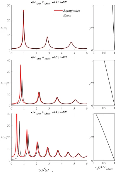
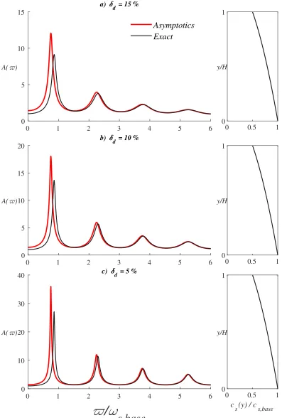
bedrock (Nt h layer) . . . 43 3.4 Base-to-top dynamic amplification A($)(with corresponding

verti-cal S-wave profilecs(y)), comparison between eq. (3.17) (Exact) and eq. (3.22) (Asymptotics) for inhomogeneity factorn=0.1 . . . 50 3.5 Base-to-top dynamic amplification A($)(with corresponding

verti-cal S-wave profilecs(y)), comparison between eq. (3.17) (Exact) and eq. (3.22) (Asymptotics) forn=0.5 andβ =0.5, analysis of damping

sensitivity . . . 53 3.8 Scheme of wave propagation in heterogeneous soil resting on rigid

(10)

3.9 Base-to-top dynamic amplification A($)(with corresponding verti-cal S-wave profilecs(y)), comparison between numerical solution of eqs. (3.2) and (3.3) (Exact) and eq. (3.32) (Asymptotics) . . . 61 3.10 Base-to-top dynamic amplification A($)(with corresponding

verti-cal S-wave profilecs(y)), comparison between numerical solution of eqs. (3.2) and (3.3) (Exact) and eq. (3.32) (Asymptotics) . . . 63 3.11 Comparison of fundamental frequency: roots of denominator of

eq. (3.22) (Asymptotics), eq. (3.39) (Rayleigh Q.), roots of denomi-nator of eq. (3.17) (Exact) . . . 64 3.12 Schematic representation of two possible equilibria (red = inertial

forces, green = damping forces, blue = elastic forces , orange = external load). . . 65 3.13 Transfer function and profile corresponding to KiK-net sites

(discon-tinuous line marks the estimate eq. (3.50)). . . 73 4.1 Schematic representation of a representative cross-section of the

sys-tem being surveyed, including some relevant parameters . . . 79 4.2 Scheme of the Younan-Veletsos problem (expressed in total

displace-ment) . . . 92 4.3 Scheme of the Younan-Veletsos problem (expressed in relative

dis-placement) . . . 93 4.4 Scheme of probe location for “vertical displacement at the top of the

wall” . . . 95 4.5 Transfer function for the vertical displacement at the top of the wall,

ν =0.1,δd =0.16 . . . 96 4.6 Transfer function for the vertical displacement at the top of the wall,

ν =0.1,δd =0.05 . . . 96 4.7 Transfer function for the earth thrust the wall,ν =1/3,δd =0.01 . . 97 4.8 Transfer function for the earth thrust the wall,ν =0.1,δd =0.05,0.1,0.2 98 4.9 Three regions in the Younan-Veletsos problem: dark grey is the

narrow layer around the wall controlled by the boundary conditions, light grey is the transition region and white the far-field . . . 101 4.10 Contour to be used to evaluate the path-independet integrals . . . 108 4.11 Schematic representation of excavation within soil resting over rigid

bedrock . . . 111 4.12 Exact solution of the quasi-static thrust derived from eq. (4.14) and

(11)

5.1 Comparison of quasi-static vertical displacement at the top of the

wall: eq. (4.15) (Exact), model outcome andAbaqus(FEM) . . . 126

5.2 Comparison of quasi-static earth thrust: eq. (4.14) (Exact), exact solution for two-wall system (Wood (1973)), model outcome and Abaqus(FEM) . . . 127

5.3 Comparison of quasi-static earth thrust: eq. (4.14) (Exact), model outcome and result in [KLM12] using sinusoidal shape. . . 127

5.4 Comparison of dynamic earth thrust: eq. (4.14) (Exact), model out-come using κqs(ν)andκ(ν, $)(ν =1/3) . . . 128

5.5 Comparison of dynamic earth thrust: eq. (4.14) (Exact), model out-come using κqs(ν)andκ(ν, $)(ν =0.1) . . . 129

5.6 Comparison of dynamic vertical displacement at the top of the wall: eq. (4.14) (Exact), model outcome usingκqs(ν)andκ(ν, $) . . . 130

5.7 Comparison of dynamic κ(ν, $) and quasi-static κqs(ν) compress-ibility factors . . . 130

6.1 Scheme of the problem to be considered including the contour used to evaluate conservation laws . . . 134

6.2 Comparison between expression provided by Conti and collaborators and the outcome of the proposed model for ν = 0.4 and different values of aspect ratio . . . 146

C.1 System re-framed in terms of relative displacements . . . 173

C.2 System after assuming harmonic excitation and response . . . 174

C.3 System after non-dimensionalization . . . 175

C.4 Nondimensional system after applying symmetry argument . . . 176

C.5 Comparison for the quasi-static vertical displacement: exact, model and asymptotitc of exact solution . . . 184

C.6 Scheme of LADWP reduced problem I . . . 185

C.7 Scheme of LADWP reduced problem II . . . 187

D.1 Gibbs phenomenon observed when using sin(knη)to expand 1 in the intervalη∈ [0,1] . . . 191

(12)

LIST OF TABLES

Number Page

3.1 Error (%) in estimation by eq. (3.22) of the natural frequency

corre-sponding to the three first resonance peaks . . . 54

3.2 Error (%) in estimation by eq. (3.22) of the amplitude corresponding to the three first resonance peaks . . . 54

3.3 Error (%) in estimation by eq. (3.22) of the amplitude corresponding to the three first resonance peaks for different values of damping . . . 55

3.4 Error (%) in estimation by eq. (3.22) of the natural frequency cor-responding to the three first resonance peaks for different values of damping . . . 55

3.5 Amplitudes at the fundamental mode in figs. 3.4 to 3.6 . . . 70

3.6 Information concerning KiK-net site IBRH17 . . . 71

3.7 Information concerning KiK-net site TKCH08 . . . 71

3.8 Information concerning KiK-net site IBRH10 . . . 72

4.1 The n-physical parameters of the soil-structure-interaction problem to be considered through dimensionless analysis. . . 83

4.2 Characteristic values of physical parameters of the soil-structure-interaction problem and corresponding range of dimensionless groups. 89 4.3 Base parameters used in finite-element simulations . . . 94

6.1 Summary of contributions to the PII . . . 140

6.2 Summary of contributions to the PII, in terms of stresses . . . 140

6.3 Summary of contributions to the PII, in terms of displacements and displacement gradients . . . 141

6.4 Summary of simplified contributions to the PII, in terms of displace-ments and displacement gradients, unknowns highlighted in color. . . 143

6.5 Summary of contributions to the PII, in terms of stresses, unknowns highlighted in color. . . 143

6.6 Summary of contributions to the PII, in terms of stresses, unknowns highlighted in color. . . 144

(13)

C h a p t e r 1

INTRODUCTION

This first chapter aims to provide the reader with:

• Brief introductions to both soil-structure interaction and path-independent integrals, and motivation for the need of applying the second to the first.

• Objectives and scope of this text.

• Organization of the text.

• A list of supplementary materials.

1.1 Soil-structure interaction: a primer

By and large, civil structures are either partially or completely embedded in the soil. The soil, in and of itself, is an intricate system, made up of a large collection of microconstituents which interact with each other through (in general) contact forces, with either air or water filling the void spaces between them. These microconstituents are usually referred to as grains, although clayey soils display a more complex microstructure.

Due to the inherent uncertainty when dealing with it, civil engineers tend to avoid direct consideration of soil-structure interaction effects when designing or analyzing a structure, indirectly accounting for it by increasing safety margins. However, this procedure is unfeasible whenever the structure bears special standing (critical infrastructure, e.g., a nuclear power plant) or its value is deemed somewhat too high for the risk to remain unaccounted. A paramount source of peril is, of course, seismic activity.

(14)

to the wave scattering produced by the presence of the structure, which is “seen” as an obstacle by the impinging wavefront. Such an event is labeled askinematic interactionin SSI lexicon.

On the other hand, the coupling between structure and soil response (in particular for relatively soft soils) can trigger a pernicious cycle of increasing inertial forces in the structure, which induce larger deformations in the soil surrounding the structure or its foundation, and in turn may provoke further deflection and accelerations in the structure. This effect is labeled, in SSI, asinertial interaction.

The approaches to study the SSI phenomenon have ranged from analytical inves-tigations, forerunners tracing back to the nineteenth century [Cer82; Bou85], to numerical simulations and experimental work.

The original push towards anchoring SSI as a discipline within Solid Mechanics saw initial successes [Ter16; Lov29], many of them supplied by the Austro-German tra-dition headed by Terzaghi [Kau10]. These first attempts were concerned with statics and aimed at obtaining the response of a linear-elastic half-space subjected to differ-ent types of loads applied at its free-surface. Equivaldiffer-ent problems in dynamic SSI have exhibit more difficulties than their quasi-static counterpart, as was expected. A collection of available solutions can be found in Kausel’s compendium [Kau06]. The basic conceptual framework to understand this phenomenon is attributed to Prof. George Housner, who penned two milestone articles (the first one in collab-oration with Prof. R.G. Merrit), [MH54; Hou57b], by the mid 1950s, wherein he explained the effect of man-made structures on the displacement field at the ground surface elicited by earthquakes. Once the conceptual pieces of the phenomenon were ascertained, simple-yet-insightful reduced models describing the main traits of the interplay between soil and structure were proposed by [SRW72], leading up to current practice recommendations codified, in the US, by the National Institute of Standards and Technology (NIST) [NIS12].

(15)

allow for the incorporation of more realistic material behavior than linear elasticity; as a token, see [Ana+08]. Results such as those provided by Prof. Gazetas [Gaz91] are already common tools in the trade. Regrettably, numerical parametric studies display limited capacity in assessment of the underlying physics and caution must be exercised when interpreting and extrapolating results from parametric analyses.

For more detail on both analytical and numerical work, the reader is referred to the comprehensive survey curated by Prof. Eduardo Kausel [Kau10].

Experiments remain the touchstone of scientific endeavors and the ultimate arbiter of suitability of engineering mdoels. Regarding SSI, efforts in the experimental front have been vexed by another factor: in reality, the soil is tantamount to a granular medium and not so much to a linear-elastic material. For the most part, analytical results in dynamic SSI are restricted to linear-elastic medium, and so are the aforementioned milestones in numerical work. This has hindered the reconcil-iation between these and experimental results [GS91], albeit it seems possible to find mechanical parameters so that the analytical and numerical methods can agree with the experiments [Sey+18]. On the bright side, profuse instrumentation of both buildings and sites [GAG19; Oka+04] is common in seismic areas nowadays, grant-ing researchers with access to a large database amenable to gauge the accuracy of their models.

In any event, the push continues in all fronts, propelled by the necessity of assessing complex scenarios and systems that demand novel tools or deeper understanding.

The spark that initiated the work in this text was the construction of the Head-works Reservoir, in Los Angeles, California [Hud+14]. These 110-million-gallon (combined total) reinforced concrete structures posed, due to their singularity, a phenomenal design challenge on the Los Angeles Department of Water and Power (LADWP) and onerous economic effort to the State of California and its citizens. This remarkable project motivated a re-examination of the SSI physics concerning water underground water reservoirs subjected to seismic action [Hus+16a] as well as the available guidelines and numerical design tools [Har+14]. The inception and a sizeable part of this thesis may also be ascribed to this endeavor.

1.2 Path-independent integrals in Continuum Mechanics and its potential for solving problems in soil-structure interaction

(16)

[image:16.612.157.457.69.270.2]

Figure 1.1: Aerial view of Headworks Reservoir (under construction, 2018). Image credit: Los Angeles Dept. of Water and Power (downloaded from ladwpnews.com/epk-headworks-reservoir-construction)

divided by ambit (quasi-static or dynamic regime) and ordered chronologically. At the end of this section we will motivate the aptitude of these PII as useful tools to untangle problems in Soil-Structure Interaction.

1.2.1 The origins: quasi-static Fracture Mechanics

Eshelby is recognized as the first researcher that found a surface-integral representa-tion for “force on an elastic singularity or inhomogeneity” [Esh56], in 1951 during the course of his studies on lattice defects, although an immediate antecedent can be found in the Peach-Kohler equation [Lub18], obtained one year earlier. Eshelby did note that in the absence of defects his result represented a conservation law for regular small-deformation elastostatic fields in homogeneous yet not-necessarily-isotropic bodies. Besides, he acknowledged that this result could be extended to finite kinematics.

(17)

the domain and the to-be-understood regions, without needing to solve the field equations of the problem. The J-integral is nothing but a particular instance of a more general theory, of which the aforementioned work by Eshelby was but another example.

The equivalence of these results as well as a general theory of generalized con-servation laws expressed in terms of path-independent integrals over elastic bodies was presented by Knowles and Sternberg [KS72], for both infinitesimal and finite kinematics, wherein it was also highlighted how these conservation laws relate to the classic Noether’s theorem of mathematical physics [Bye98]. A similar text, which did not foresee connections to fracture, had been published by Günther previously [Gün62] in German, what hindered the dissemination of the findings to the extent that they had to be re-discovered independently a decade later.

Chen and Shield [CS77] explored a number of conservation laws in elastostatics connected to different types of strain-energy functionals. Moreover, they provided equivalent identities relating two different states, an approach that was later system-atized by Zhang and Achenbach [ZA89], who also presented the so-called Boundary Integral Method (BIM).

Rice [Ric85] also noted the extent to which these relations resemble the classic Maxwell relations from Thermodynamics, both in appearance and content: the con-served integrals represent “energetic force” related to invariant transformations. One can find a “translational integral” (the J-integral itself, related to loss of translational symmetries), a “rotational integral” (the L-integral, related to loss of rotational sym-metries), and a “scaling integral” (the M-integral, related to infinitesimal changes of scale). It was also acknowledged that the work done by these forces represents dissipation in accordance to the Second Law of Thermodynamics, and that then, logically, these become useful to establishevolution criteria(e.g. crack growth).

(18)

1.2.1.1 The extension to the dynamic setting

These path-independent integrals were originally intended to help deal with static or quasi-static problems, and their extension to more general dynamic settings was challenging: these path-independent integrals are intimately related to the elliptic nature of the static problem, such ellipticity being lost as one moves into the dynamic realm and appearance of inertial terms turn the equations hyperbolic and wave propagation phenomena take precedence.

Nevertheless, this issue was shown to be avoidable, as new dynamic approaches were developed to deal with problems in Dynamic Fracture Mechanics [Fre98], a logical extension of the pioneering work carried out by Rice and others.

Nilsson [Nil73] noted that translating the problem to the frequency domain, by means of application of Laplace’s transform that would turn the original hyperbolic field equations into elliptic field equations (the inertial forces become regular body forces proportional to the displacement), which enables the definition of path-independent integrals relevant to the dynamic setting yet with a caveat: one is bound to interpret the results, firstly, not in the time domain but rather in the frequency domain. Once the results in frequency domain have been obtained, the Laplace’s transform must be inverted in order to finally obtain results in time domain. That inversion can be expressed as the convolution of the product, and so was noted by Gurtin [Gur76] .

Nilsson’s approach also hints at yet another way of dealing with the dynamic prob-lem: assuming harmonic forcing and either neglecting free-vibration or assuming steady-state conditions, then, by virtue of linearity, the system of hyperbolic equa-tions yield a system of elliptic equaequa-tions wherein the unknowns are the (complex) amplitudes of the harmonic response. This framing is customary in the study of cracked bodies subjected to harmonic loading.

The literature in the field has increased dramatically, and it is beyond the scope of this text to delve too much into it. The reader in search of further details is referred to Prof. Maugin historical survey [Mau13], see Chapter 14 particularly, or to the monograph on configurational forces by the same author [Mau16], as well as Dynamic Fracture Mechanics monograph by Prof. Freund [Fre98], which remains an invaluable reference.

(19)

there exist many other applications of these path-independent integrals as work on this field has been steady during the last years insofar different flavours of continuum mechanics are concerned: strain discontinuities in solids [AK90] and phase transitions [AK93], just to name a few. Reasons for this positive turnout will also be given in the next section.

1.2.2 On an analogy between Fracture Mechanics and Soil-Structure Inter-action: configurational forces

Despite the progress made in many branches of Continuum Mechanics by mediation of these path-independent integrals, geomechanics has remained untouched by them.

The might of the path-independent integrals resides, first and foremost, in its intrinsic capacity to reveal meaningful interrelations between different regions in the same domain, intertwining the response of those regions that are more complex to the one of those that are simpler to understand and assess. Therein their usefulness for fracture is found, as they allow to coonect the complex local response at the crack, which is hard to assess, to the pre-established, already-understood, loading conditions.

(20)

or electric charge, neither of them present in either the crack or the dislocation). In the absence of sources or sinks, these balance laws may as well be dubbed conservation laws.

The prior relation between the crack and the plate, or between the regular atomic lattice and the dislocation, can forthrightly be mapped to a structure surrounded by soil: the presence of the structure (either a foundation, a pipe, an excavation...) alters the symmetry of the soil domain (in other words, introduces an heterogeneity). Hence, the path-independent integrals establish a relation between the response at thefar-field, the region far from the structure/inclusion (which is simpler to analyze and plays the role of the known loading condition in the analogy to fracture) and thenear-field, viz. the region of the soil domain surrounding the inclusion (which plays the role of the crack tip in the analogy). Let us also link the prior discussion on dislocations to the presence of a man-made structure on ground, a foundation for instance. Even before considering the mass or the stiffness of the structure, one can recognize that it does represent a change in the geometrical configuration in an otherwise homogeneous system, and thus it is as if there was a kind ofdefectwithin the material. Now consider some sort of excitation on the whole system, say, an earthquake. The whole system moves, but the zone around the foundation (near-field) moves differently compared to the rest of the soil, and thus we may say some extra force, that does not appear anywhere else, is being applied to it and changing the configuration locally. These configurational forces can be devised through the path-independent integrals (the new conservation laws), as we have already mentioned and we shall illustrate. Of course, this phenomenon has to represent a new rendition of thekinematic interactionphenomenon that was introduced in the previous section.

Besides, adding mechanical properties and mass to the foundation would bring other forces (internal elastic, inertial) into the picture, but the configurational force will remain.

We present yet one more item upon which the analogy could be extended: see how, as in the case of the crack tip, the work of the thermodynamic forces is a dissipation term, then, what about the underground structure? The dissipation mechanism in this case must be theradiationassociated with the scattered wavefield.

(21)

comprehension of problems like those that concern us.

Finally, we should notice that these conservation laws can be of much utility even when there is no structure but just changes within the soil domain. We surmise that changes in stratigraphy, slopes, and other common geomechanical affairs may be also studied from the viewpoint of PII.

1.3 Objectives and scope

This thesis chief objective is motivating and illustrating the potential of path-independent integrals, developed originally in the ambit of Fracture Mechanics, for analyzing SSI problems, which appears to have gone unexplored.

To make this precise, we shall focus first on the problem considered by Dr. Younan and Prof. Veletsos in two landmark papers [VY94b; VY94a], which we shall refer as the Younan-Veletsos problem from this point onward. We shall show how considerations derived from PIIs help elucidating relevant features in the problem. In the course of study of the Younan-Veletsos problem, we will provide the exact solution of the problem with smooth-rigid walls, complementing the classic solution obtained by Wood for a system with two of these walls [Woo73]. We must clarify that this solution is given in wavenumber space, since the inversion of Fourier transform that allows moving from wavenumber back to spatial coordinates has not been achieved yet. Nevertheless, this shall not prevent us from evaluating some relevant parameters, as the earth thrust, numerically.

Another basic application of PII to a more complex problem, namely a reservoir within a thick soil layer resting on soil, shall also be demonstrated. In spite of requiring the introduction of a number of simplifying assumptions, the result is deemed interesting, as it shows how the PII can be used to obtain bounds of certain parameters in geometric configurations that do not lend themselves to finding a simple closed-form solution. This result can be considered a first attempt towards an answer of a rather general and consequential question: how much information onmechanicalforces acting on a certain certain can be retrieved from the analysis ofconfigurationalforces?

(22)

Additionally, there are a number of ancillary topics addressed in this text.

One of them consists of providing a general framework wherein the problem of seismic response of underground water reservoirs can be assessed. The chosen instrument to fulfill this effort is none other than Dimensional Analysis, as outlined by Buckingham’s Pi Theorem [Lan51]. We shall put forward a descriptive model of this scenario, including a bevy of parameters describing the response of soil, water, and structure, as well as features of the seismic load. Once this is done, we shall interpret the physical significance of the dimensionless groups that derive from this set of parameters. Once the meaning of each has become apparent, we shall map specific configurations of the physical configuration to distinct points in the parameter space. We hesitate referring to this contribution as novel, since it so appears that the use of Dimensional Analysis is gaining standing among theoreticians in our field of Geotechnical Earthquake Engineering; here one must mention a notable paper by Prof. Conti and collaborators [CMV17]. We must also mention that the comparable section in this text was written prior to the author being aware of their work. In a private communication, Prof. Conti rightly pointed out that this wherewithal has already been used extensively by experimentalists in the field [Woo14].

Another relevant theme in this thesis has been One-dimensional Site Response (1D-SR). Devoting a full chapter to the topic in a thesis primarily concerned to SSI may seem an unnecessary digression at first, but this is far from being the case, as there are good reasons to do so. First and foremost, due to its relation to SSI (far-field analysis). Moreover, in and of itself, it is a relevant problem that concerns geotechnical engineering experts as much as SSI, and it has some unexpected ramifications [Gaz87]. We shall focus on two questions: how to characterize, in first place, the high-frequency response of sites, and secondly, idem for the fundamental resonance mode. This front has been limited 1D-SR, and the extension of the conclusions to SSI is a pending task, although we already provide some results bearing direct consequences to SSI recommendations [NIS12].

The scope limitation of the results will be thoroughly discussed in the text, especially with aid of the dimensionless groups that we devise to characterize the problem of seismic response of underground reservoirs.

(23)

1.4 Organization of the text

Chapter 2 considers the basic theory Elasticity and Elastodynamics, including Path-independent integrals, necessary for upcoming discussion. In addition, fundamen-tals of soil behavior and 1D Site Response are revisited.

Chapter 3 is concerned with new results in 1D-SR. These range from explicitly presenting and displaying interrelations between the two possible manners of con-ceptualizing the problem when there exists rigid bedrock (i.e. in terms of either relative or total displacements), to a characterization of the high-frequency regime and the first resonant mode in these systems. The consequences of these results for SSI are not included in the text as they are still in the early stages, but relevant comments on the matter are included by the end of the chapter.

Chapter 4 presents an overarching study, assisted by Dimensional Analysis, of seismic response of underground water reservoirs. Thorough discussion of the different parameters and regimes in the problem is pursued. Then, the main object of study, the Younan-Veletsos problem, is presented, solved, and its main qualitative features discussed. Finally, a relaxation of the Younan-Veletsos problem, wherein there is soil between structure and bedrock, is considered in the long-wavelength regime, and, providing certain conditions, a bound for the earth thrust is derived in terms of the far-field response.

Chapter 5 delves into how to use the insight from PIIs and the qualitative features of the problem to propose a new simplified model that captures most distinct features of the exact solution. Such a model is proposed and compared to the new exact solution and to other simplified models.

Chapter 6 is occupied with developing a new framework to understand soil-structure kinematic interaction within the theory of configurational forces. A simple model for foundation input motions is drawn out from the general expressions and compared to the classic results by Elsabee and Morray [EMR77].

Chapter 7 provides conclusions and outline future research avenues.

(24)

1.5 Supporting material

In an effort to ease the dissemination of the findings contained in the text, a number of Mathematica [Wol00] notebooks are provided as supporting material. These contain details on derivations and also implement the main results of this study. A list, including brief description, of these notebooks follows:

• “Chapter3 1D Site Response.nb" was used to generate the transfer functions displayed in plots for Chapter 3.

• “Chapter4 Exact Solution YV Problem.nb” contains some details of the derivation of the main result in the chapter, as well as implementation of the exact solution of the problem being considered. This notebook can be used to generate the data displayed in figures in Chapter 4.

• “Chapter5 Evaluation Dynamic J Integral.nb”,likewise, implements and eval-uates the results in Chapter 5.

• “Chapter6 Kinematic Interaction.nb” was used to generate the main results in Chapter 6 (namely those contained in Figure 6.2).

(25)

C h a p t e r 2

BACKGROUND

Here we aim to present the fundamentals upon which the upcoming study hinges:

• Modeling of soil as linear-elastic material.

• Elastostatics and Elastodynamics, including Williams solution for notches.

• Variational formulation in Continuum Mechanics (due to its relevance to path-independent integrals).

• Path-independent integrals.

• One-dimensional site response.

2.1 The soil as a linear-elastic medium and its dynamic properties

The constitutive law used to describe the soil response poses a bottleneck to any effort of predicting response of soil-structure systems. As the customary saying goes, the accuracy of predictions by a model can be as good as, but not better than, the material description one adopts. Accordingly, finding a simple-yet-accurate constitutive relation to describe the soil behavior is paramount.

In general, most clays, silts, and sands present a linear stress-strain relation up to strains ∼ 10−4 [PD74], although for some peculiar clay types the range can be extended up to ∼ 10−3 [DV87]. Let us keep these orders in magnitude in mind, as we shall resurface them when the discussion of range of validity of our analysis ensues in section 4.2.

(26)

only in one direction [Gib74], although oftentimes it tends to be ignored. In our work, we shall consider, whenever necessary, either that the depth is not excessive so that the degree of anisotropy remains small, or that the wave propagation elicits response in just one direction. Should there be cases such that neither suppoition is possible, our results must be interpreted as limited to specific materials whose properties are such that it can be considered isotropic.

Another concern is how to model internal dissipation in the granular material from amacroperspective. An unvarnished way to accomplish this would be considering soil as a viscous medium where dissipation is proportional the deformation rate; experiments contradict this last assertion, though. Dissipation in most soils subjected to cyclic load follow from an hysteresis loop that appears to be proportional to deformation amplitude instead of rate, and dissipation is present at even very low strain levels [Kra96]. Besides, confinement pressure has been proved to affect dissipation too [IZ93].

The customary, simple approach of adding this dissipation is through aloss factor, turns the elastic constants from real parameters to complex parameters, as it adds a factor (1+ iδd), δd (real number, also referred to as hysteretic damping factor, sometimes appearing with an extra factor 2) will be adopted (“i” is the imaginary unit). Note that this approach is limited to frequency-domain analyses.

2.2 Elastostatics

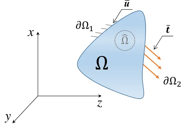
Before starting, a word on notation: bold symbols represent vectors and tensors, Einstein’s index convention is in effect, unless otherwise stated, we shall use the letters x, yandz to refer to indices, and thus, for instance, the displacement vector can be equivalently expressed as u = ui = [ux,uy,uz]> = [u,v,w]>, the second triad (u,v,w) shall be used whenever referring to specific components directly.

We begin by considering an homogeneous body occupying a domainΩ⊂ _R3_which

undergoes deformations elicited by external loads and prescribed displacements. The boundary of the domain is referred to as∂Ω= ∂Ω1∪∂Ω2(such that∂Ω1∩∂Ω2 =

). As a cardinal assumption, this problem will be framed using infinitesimal kinematics. Moreover, in this section we shall consider deformation rates such that the inertial forces appearing anywhere within the body happen to be negligible. Let

(27)

conditions governing the evolution of the system:

i j = 1

2

∂ ui ∂xj +

∂uj ∂xi

inΩ, (2.1)

σi j,j+ρbi =0 inΩ, (2.2)

σi j = _∂∂W ui,j

inΩ, (2.3)

u = u on∂Ω1, (2.4)

σi jnj = ti on∂Ω2, (2.5)

whereW(x)represents the corresponding strain energy density,nj is the outwards-facing normal. Thermal considerations are intentionally left out of the picture, as these are irrelevant for the problems we shall focus on.

x

𝜕Ω

u

𝒕̅

𝜕Ω

Ω

y

[image:27.612.158.451.299.501.2]

z

Figure 2.1: Scheme of the boundary-value problem

If we were to add the hypothesis of linear material response, then

W = 1

2σi jεi j. (2.6a)

If we allow for elastic (anisotropic) behavior

W = 1

2ci j klεi jεkl, (2.6b)

ci j kl being the tensor of elastic constants (which must satisfy the symmetry con-ditions ci j kl = cjikl = ci jl k = ckli j). If eq. (2.6b) holds, it implies the so-called anisotropic Hooke’s (constitutive) law:

(28)

which in turn can be generalized to heterogeneous media by rendering the elastic constants function of the position,

σi j(x)= ci j kl(x)εkl(x). (2.8)

Combining eq. (2.7) and eq. (2.1) into eq. (2.2), the Navier equations (formulation in terms of displacements) are obtained, moreover, they can be also used into Equation (2.5) to express the traction boundary conditions in terms of displacement gradients as well, hence the problem defined by eqs. (2.1) to (2.5) becomes

(ci j kluk,l),j +ρbi = 0 inΩ, (2.9)

u=u¯ on∂Ω1, (2.10)

(ci j kluk,l)nj = ti on∂Ω2. (2.11)

This problem belongs in the category of linear-elliptic boundary-value (mixed boundary conditions) problems, made up by systems of partial differential equa-tions. Solution existence and uniqueness are not guaranteed. We shall, nevertheless, from this point forward, assume that any condition that existence and uniqueness necessitate are granted.

Finally, if the material is homogeneous and isotropic, then the tensor of elastic constants must be of the form

ci j kl =λ δi jδkl +µ(δikδjl +δilδj k), (2.12) where δi j represents the Kronecker delta tensor and λ, µ(shear modulus) are the “Lamé constants” of the isotropic material. It suffices to setλ(x)and µ(x)in order to consider a material that is isotropic yet heterogeneous.

Using eq. (2.12) in eq. (2.6b) becomes

W = µ εi jεi j + 1

2λ(εk k)

2_, _(2.13)

whereas eq. (2.6b)

σi j = 2µεi j +λεk kδi j = µ(ui,j+uj,i)+λuk,k, (2.14) and eqs. (2.9) to (2.11)

µui,j j +(µ+λ)uj,i j +ρbi = 0 inΩ, (2.15)

u= u¯ on∂Ω1, (2.16)

_µ

(ui,j +uj,i)+λuk,kδi j

(29)

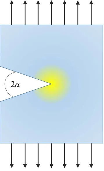
2.2.1 Stress concentration at corners: Williams Solution

It is well-known that the linear elastostatic stress field, and the linear elastodynamic one too [Fre98], around a crack tip is singular, and the singularity scales as the inverse of the square-root of the distance from the crack-tip.

The foregoing does not preclude other configurations from presenting different singular stress fields; actually, any configuration with sharp-edge intersections (a corner or a notch) will present a stress singularity at the intersection, albeit its scaling will not be “as singular as” the one of the crack tip.

The linear-elastic stress concentration at notch tips was settled by Williams [Wil52] (himself a Galcit graduate).

[image:29.612.217.396.282.577.2]

2 α

Figure 2.2: Notch scheme

(30)

We will consider a configuration with rectangular corners in both section 4.4 and Chapter 6, that is, configurations corresponding to α = π/4 (see fig. 2.2), hence σi j ∼ r−0.495, where r represents distance from the tip of the corner. When it comes to consider contour integrals around these domains, the customary approach is to add a circumferential contour enclosing the singularity (so that no elastic singularities are enclosed in the domain). In such scenario, it is easy to realize that the contribution of this piece of contour to both the stress integral (the thrust) and to the integral of the energy-momentum tensor (proportional to the square of the stresses, to be formally presented in section 2.5.1.1) vanishes as the radius of the circumference tends to zero. The latter is due to the perimeter contour tending to zero as ∼ r whenr → 0 whereas the integrand scales, in this case, no faster than ∼ (r−0.495)2 asr → 0; thus, in the limit, the whole integral goes as r1−2·0.495 → 0 (although very slowly) since the exponent is still positive (note that the same happens for any notch except whenα= 0, that is, the crack is recovered and the contribution of the integral of the energy momentum tensor over the infinitesimal contour is finite [Ric68]).

Acoording to Luco [LW72], a similar result abscribed to the problem of settle-ments of rigid foundations was derived by Muskhelishvili [Mus13] and by Abramov [Abr37] independently.

2.3 Elastodynamics

Let us lift the restriction on negligible inertial forces. Time,t, enters the formulation explicitly as an independent variable. Hence, now we seek displacements u = ui(x,t), strainsε = εi j(x,t)and stressesσ= σi j(x,t)satisfying the field equations and boundary conditions governing the evolution of the system:

εi j = 1

2

∂ ui ∂xj +

∂uj ∂xi

=u(i,j) inΩ, (2.18)

σi j,j+ ρbi = ρuÜi inΩ, (2.19)

σi j = ∂W

∂ui,j

inΩ, (2.20)

u =u on∂Ω1, (2.21)

σi jnj =ti on∂Ω2. (2.22)

(31)

Following the same the chain of assumptions that lead us to the (quasi-)static definition of the elastic problem in terms of displacements, eqs. (2.9) to (2.11), we can reach their dynamic analogue:

µui,j j +(µ+λ)uj,i j +ρbi = ρuÜi inΩ, (2.23)

u=u¯ on∂ωs, (2.24)

_µ

(ui,j+uj,i)+λuk,kδi j

nj = ti on∂Ω2. (2.25)

Basically, the only difference is that inertial forces have to be added to eq. (2.15) so that the equilibrium in the bulk of the body is achieved among internal forces, external body forces, and the supplementary action of inertial forces, eq. (2.23).

At this point, let us introduce the Cartesian frame of reference that has been implicit so far. This, the position vector comes defined asx =[x, y, z]>, and eq. (2.23) can be expanded into

µ

∂2_u

∂x2 +

∂2_u

∂y2 +

∂2_u

∂z2

+(λ+ µ) ∂ ∂x

∂ u

∂x +

∂v

∂y +

∂w

∂z

+ ρbx = ρ ∂2_u

∂t2 , (2.26a)

µ

_∂₂ v

∂x2 +

∂2_v

∂y2 +

∂2_v

∂z2

+(λ+ µ) ∂ ∂y

_∂ u

∂x +

∂v

∂y +

∂w

∂z

+ ρby = ρ

∂2_v

∂t2 , (2.26b)

µ

∂₂ w

∂x2 +

∂2_w

∂y2 +

∂2_w

∂z2

+(λ+ µ) ∂ ∂z

∂ u

∂x +

∂v

∂y +

∂w

∂z

+ ρbz = ρ ∂2_w

∂t2 . (2.26c)

Note that we do not have an elliptic problem anymore, so now the problem belongs to the linear-hyperbolic class.

2.3.1 Plane-strain elastodynamics

(32)

Let us assume that z = 0 represents such symmetry plane, and that there are no forces whatsoever nor gradients of any kind along its normal direction. Under these suppositions, it follows thatu,z = v,z =w,z = 0 andw =0 itself at this representative section (recall thatσ33 =λ(u,x+v,y),0 necessarily), eq. (2.26c) is trivially satisfied

and eq. (2.26a) simplify into

(λ+2µ)∂2u

∂x2 +(λ+µ)

∂2_v

∂x∂y +µ

∂2_u

∂y2 +ρbx = ρ

∂2_u

∂t2 , (2.27a)

(λ+2µ)∂2v

∂y2 +(λ+µ)

∂2_u

∂x∂y +µ

∂2_v

∂x2 + ρby = ρ

∂2_v

∂t2 . (2.27b)

2.4 Variational formulation of Continuum Mechanics

In some systems, it is acknowledged that the observed states coincide with those that extremize a certain functional defined over the variables describing the system. For such systems, it is said that its evolution is governed by anextremum principle. Moreover, in even more general terms, for some systems the observed state are identified as stationary points of a certain functional, this it is said that the system abides by a stationarity principle. See that extrema are stationary points, and stationary points that are not extrema are referred to assaddle points.

Consider a functionalΦ: X → _Rof the form Φ[u]=

∫

Ω

W(x,u,∇u)dV + ∫

∂Ω2

F (x,u)dS, (2.28)

whereXis an affine space referred to as the space ofadmissible solutions. Consider

V to be the translational space of X, which is itself a linear space, and is referred to as the space ofadmissible variations. For our purposes, bothX andV are finite-dimensional spaces. The first variationof Φ at a point u ∈ X in the direction of

u ∈V is

hDΦ[u],ui =

d

dΦ(u+u)

=0+

, (2.29a)

since the working spaces are finite dimensional

= ∂Φ_∂ xi

(x)ui (2.29b)

hence using eq. (2.28) and integration by parts

= ∫

Ω

∂W

∂ui − ∂

∂xj ∂W ∂ui,j

uidV +

∫

∂Ω2 ∂

F ∂ui +

∂W ∂ui,j

nj

(33)

A point u ∈ X is said to be astationary pointofΦinX when

hDΦ[u],ui=0, ∀u ∈V. (2.30)

Thus, for eq. (2.30) to be verified in eq. (2.29c) both integrands must vanish for any value of the admissible variation. This condition yields the so-called Euler equationsofΦ:

∂W ∂ui

− ∂ ∂xj

∂W ∂ui,j =

0 inΩ, (2.31a)

∂F ∂ui +

∂W ∂ui,j

nj =0 on∂Ω2. (2.31b)

Satisfying these equations is a necessary condition for stationarity. Note that the definition of the equations themselves is contingent upon the capacity of defining some derivatives properly.

By this as it may, the next step is realizing that the problem defined by eqs. (2.1) to (2.5) is but the Euler equations corresponding to the stationaity condition of the celebratedHu-Washizu functional:

Φ[u,ε,σ]=

∫

Ω

W(ε)+σi j(u(i,j)−εi j) −ρbiui

dV

−

∫

∂ωs

σi jnj(ui−u¯i)dS−

∫

∂Ω2 ¯

tiuidS,

(2.32)

in this caseW =W(ε)+σi j(u(i,j)−εi j) −ρbiui andF = −(σi jnj(ui−u¯i)+t¯iui). Therefore, solving the problem posed by eqs. (2.1) to (2.5) amounts to finding stationay points of the function in eq. (2.32). Assuming the functional satisfies convexity requirements, stationarity requires the functional to be minimized with respect to the strain field, maximimized with respect to the stress field and finally minimized with respect to the displacement field:

Stationarity ⇐⇒ min

u minσ minε Φ[u,ε,σ]. (2.33) One can obtain a reduced variational principle, the so-called Hellinger-Reissner Principle, by minimizing eq. (2.32) with respect to the strain field, that is, enforcing eq. (2.3) a priori.

(34)

to satisfying eq. (2.1) and eq. (2.4) a priori. The corresponding functional is

Φ[u]=

∫

Ω

W u(i,j)

−ρbiui

dV −

∫

∂Ω2 ¯

tiuidS,

and the Euler equations are simply eqs. (2.2) and (2.5). A displacement field satisfying these equations solves the problem, but, more generally, one can also express the solution of the problem, call itu∗, directly from the variational priciple, eq. (2.34), as

u∗ =arg min{Φ[u] : u= u¯ on∂Ω2} . (2.34)

The bevy of assumptions that were leveled in section 2.2 (isotropy, heterogeneity, linearity...) have a direct translation into the specific actual architecture of Φ. In any case, see that the formulation holds.

The variational approach can also be extended to the dynamic setting, by means of the action functional

A[u]=

∫ t2 t1

(T[u] −Φ[u]) dt, (2.35) whereT is the potential energy functional:

T[u]=

∫

Ω ρ 2| Ûu|

2

dV . (2.36)

The Action Principlestates that the solution u∗(x,t) renders the action functional stationary.

Dynamic problem, as those mentioned in section 2.3, require of the Action Principle to be analyzed. However, we will not appeal to it, as there are strategies that, under some circumstances, will allow to fit the dynamic problem within the Principle of Minimum Potential Energy, eq. (2.34). These will prove more convenient for our purposes, since allow for definition of dynamic path-independent integrals without resorting to time convolutions, as we shall describe in section 2.5. Two possible manners of removing time from the equations is by either invoking Laplace’s trans-form, or by assuming the steady-state being in effect and working with amplitudes. For the latter, simply decomposeui(x,t)=uˆi(x)ei$t For example, eq. (2.23) would yield

∂σi jˆ ∂xj

+ ρ(_bˆ_i₊_$2_u_ˆ

(35)

where In conclusion, the dynamic problem can be recast as a static problem in which there exists a body force vector proportional to the amplitude of the displacements.

Conversely, the same problem can be also expressed in the so-called variational form. To do so, the potential energy of the body is redefined as

Φ[uˆ,∇u]=

∫

B

ˆ

W(∇u) − ρ

ˆ

bi+ $2

2 uˆi

ˆ

ui

dV−

∫

∂B2 ˆ

tiuîdS, (2.38) where ∂W/∂uî,j = σî j. The stationary condition for this functional corresponds to eq. (2.37); in other words, that equation is the Euler-Lagrange equation of the system.

2.5 Path-independent integrals and configurational forces

The existence of path-independent integrals, alternatively referred to as conservation laws, was spelled out by Knowles and Sternberg [KS72] for elastostatics, crystalliz-ing previous work of other scholars [Ric68; Che67; San59], and by Fletcher [Fle76], a student of Knowles, for elastodynamics. We will review the classic formulation, quasi-static in the absence of body forces [Ric85], first, and then will move to the dynamic realm.

2.5.1 Quasi-static, no body forces

As explained by Knowles and Sternberg [KS72], there areup tothree path-independent integrals in infinitesimal elastostatics: the vector J and L integral, and the scalar M

integral. These represent a total of seven conservation laws in the three-dimensional framework, four in the two-dimensional.

2.5.1.1 The energy-momentum tensor

The introduction of the Eshelby’s energy momentum tensor, E = Ei j, allows for a common treatment of all of these integrals. In the absence of inertia and body forces, the tensor is defined as 1

Ei j =Wδi j −uk,iσk j. (2.39) If, moreover, we presuppose a linear constitutive law, as in eq. (2.6a), the entries of the tensor can be expressed as

Ex x = 1 2

h

−σx x∂u ∂x +σy y

∂v

∂y +σzz

∂w

∂z +τxy _∂

u

∂y −

∂v

∂x

+τxz

_∂ u

∂z −

∂w

∂x

1_{Beware that other scholars [Mau16] define this tensors differently, as in the end they compensate}

(36)

+τyz

∂ v

∂z +

∂w

∂y

i

, (2.40a)

Exy =−

τxy

∂u

∂x +σy y

∂v

∂x +τzy

∂w

∂x

, (2.40b)

Exz =−

τxz∂u ∂x +τyz

∂v

∂x +σzz

∂w

∂x

, (2.40c)

Ey y =

1 2

h

σx x∂u ∂x −σy y

∂v

∂y +σzz

∂w

∂z +τxy ∂

v

∂x −

∂u ∂y +τxz ∂ u

∂z +

∂w

∂x

+τyz

∂ w

∂z −

∂w

∂y

i

, (2.40d)

Eyx =−

σx x∂u ∂y +τyx

∂v

∂y +τzx

∂w

∂y

, (2.40e)

Eyz =−

τxz∂u ∂y +τyz

∂v

∂y +σzz

∂w

∂y

, (2.40f)

Ezz = 1 2

h

σx x∂u ∂x +σy y

∂v

∂y −σzz

∂w

∂z +τxy ∂

u

∂y +

∂v ∂x +τxz ∂ w

∂x −

∂u

∂z

+τyz

∂ w

∂y −

∂v

∂z

i

, (2.40g)

Ezx =−

σx x∂u ∂z +τyx

∂v

∂z +τzx

∂w

∂z

, (2.40h)

Ezy =−

τxy

∂u

∂z +τzy

∂w

∂z +σy y

∂v

∂z

. (2.40i)

This tensor is not symmetric .

2.5.2 Invariance with respect to coordinate translation: the J-integral

The presence of some sort of “inclusion” within the otherwise homogeneous solid elicitsconfigurational forces, that is, energetic forces conjugated to the dissipation induced by the presence of the inclusion either on the contour or within the bulk of the domain.

The energy-momentum tensor is instrumental when it comes to consider configu-rational forces, as it allows to relate total configuconfigu-rational force within a subbody to their flux through the boundary of the subbody. The total configurational force acting on a subbodybΩ ⊂ Ωalong the i-th direction is referred to as Ji(bΩ)and it is

equal to

J(Ω)b = ∫

b

Ω

∇ ·EdV = ∫

∂bΩ

(37)

Note that, in the absence of heterogeneities or singularities insideΩ,b

Ji(Ω)b = 0. (2.42)

A couple of observations:

1) The definition of this path-independent integral only requires the existence of a stress potential (the strain energy density) as in eq. (2.3). Nevertheless, it is necessary condition for eq. (2.42) that the potential depends onε through its invariants [KS72], what amounts to guarantee stresses being invariant under rigid body movement (translation plus rotation).

2) It does not behoove the material to be linear, as in eq. (2.6a), nor isotropic eq. (2.6b) for eq. (2.42) to hold.

Alternatively, eq. (2.42) can be also expressed, with no appeal to the energy-momentum tensor, in a more suggestive manner which allows to judge the influence of applied tractions more easily

Ji =

∫

∂bΩ

(W ni−tkuk,i)dS =0. (2.43)

2.5.3 Invariance with respect to coordinate rotations: the L-integral

Likewise, one may consider configurational torques. The total configurational torque acting on the subbody is

L(Ω)b = ∫

b

Ω

x× (∇ ·E)dV, (2.44a)

and assuming, in addition, isotropic material

L(Ω)b = ∫

∂bΩ

x× (E n)dS =0, (2.44b) if there are no singularities within the body. The latter can also be expressed as

Li =

∫

∂Ωb

k ji W xknj−tpup,jxk +tjuk

dS = 0. (2.44c)

In conclusion, to attain these conservation laws, one has to accept the restrictions that yielded eq. (2.42)plusisotropic material response additionally.

2.5.4 Invariance with respect to scale changes: the M-integral

Consider a particular case of a self-similar expansion about the origin. Considering the configurational pressures associated with this scenario:

M(Ω)b = ∫

b

Ω

(38)

and assuming, in addition, linear material, as in eq. (2.6b),

M(Ω)b = ∫

∂bΩ

x· (E n)dS = 0, (2.45b) if there are no singularities within the body. The latter can also be expressed as

M=

∫

∂bΩ

W xini−tjuj,ixi−

tiui 2

dS =0. (2.45c)

In conclusion, to attain this new conservation law, one has to accept (in linearized kinematics) the restrictions that yielded eq. (2.42) plus linear (not necessarily isotropic) material response additionally.

2.5.5 Dynamic, no body forces

As mentioned in the introduction, a number of ways of using these path-independent integrals have been proposed for the last 40 years. We shall favor the customary approach utilized in analysis of crack tips of specimens subjected to harmonic loading, in which case one can work with the amplitudes of the harmonics rather than with functions that depend on time.

Note that the M-integral is absent from the analysis. As explained by Fletcher [Fle76], this integral requires a cumbersome treatment in time domain, as it includes terms that scale linearly with time. For this reason, and following common practice, this integral is disregarded in the steady-state dynamic setting.

Derivations of some results that follow, those that the author could not find in the literature, can be found in Appendix A.

2.5.5.1 Steady-state harmonic, total displacement

Let us begin by re-stating the decomposition σi j = σi jˆ ei$t and ui = uˆiei$t, and recall that the amplitudes are complex number whose phase represent the phase lag of the variable with respect toei$t. In the absence of body forces, eq. (2.37) turns into

ˆ

σi j,j +ρ$2uˆi =0, (2.46) if now we define properly anequivalentstrain-energy density as the potential meeting the relation

ˆ

σi j = _∂∂Wˆ

ˆ

ui,j

(39)

and theequivalentkinetic energy as,

ˆ

T = 1

2$

2_u_ˆ

iuˆi, (2.48)

notice that in order to render this quantity coherent with the classic definition, one should include a minus sign. See next how eq. (2.46) represents the Euler-Lagrange equations corresponding to the functional eq. (2.38), that can be written in this case as

Φ[uˆ,∇uˆ]=

∫

Ω

_ˆ

W(∇uˆ) −Tˆ(uˆ) dV −

∫

∂Ω2 ¯ˆ

tiuˆidS,

Using the same formalism as used for quasi-statics, we ca define a dynamic J-integral ˆJiand dynamic L-integral ˆLi as

ˆJi =∫

∂Ω

(Wˆ −Tˆ)ni−tˆjuˆj,i

dS =0, (2.49)

ˆ Li =

∫

∂bΩ

k ji

(Wˆ −Tˆ)xknj −tˆpuˆp,jxk +tˆjuˆk

dS =0. (2.50)

For eq. (2.50) to hold, it is required the material being isotropic.

2.5.5.2 Steady-state harmonic, relative displacement

For our purposes, oftentimes it will be useful to introduce a change of variables to consider time-varying imposed boundary conditions. Such change of variable consists of expressing the displacement field as relative displacements with respect to an uniform displacement field that also oscillates harmonically in time.

In other words, we shall consider the substitution ˆui → uˆi + Xi in the previous conservation laws. Note that, by our very own choice, these Xi do not depend on the spatial variables. We grant this may not be the most general case that one can consider, but it is the very one we need for subsequent work. See that, sinceXidoes not change in space, new terms do not appear along gradients of displacements, but wherever straight amplitudes are relevant, that is, in the kinetic energy. In the same fashion asXiwas introduced, we may also useXÜi =−$2Xi, where, recall,$is the frequency of the harmonic under consideration.

Then, these steady-state dynamic J and L integrals are expressed in terms of relative displacements as

ˆJi =∫

∂Ω

h

ˆ

W −Tˆ+ ρXÜluˆl

ni−tˆjuˆi,j

i

dS = 0, (2.51)

ˆ Li =

∫

∂Ωb

k ji h _Wˆ −Tˆ+ ρXÜluˆl

xknj−tˆpuˆp,jxk+tˆj(uˆk+ Xk)

i

(40)

now ˆuhas to be understood as the amplitude of the relative displacement.

2.5.5.3 Quasi-static approximation enabled by relative displacement

Finally, the quasi-static peers can also be formally obtained from eqs. (2.49) and (2.50), by assuming an expansion of the variables in terms of a small pa-rameter [BO13] that can represent either the quotient between the frequency of the harmonic load over a characteristic frequency or the ratio between a characteristic geometric length in the problem over the wavelength of the wave in the domain. The leading order term of such expansion is understood as the imposed displacement at the border that was introduced in the previous section. First, eq. (2.49) yields

ˆJi =∫

∂Ω

h

ˆ

W+ ρXÜluˆl

ni−tˆjuˆi,j

i

dS = 0, (2.53)

while in eq. (2.50),

ˆ Li =

∫

∂Ωb

k ji h _Wˆ ₊ _ρ_XÜ luˆl

xknj −tˆpuˆp,jxk+tˆj(uˆk+ Xk)

i

dS =0. (2.54)

When deciding if using or not these low-frequency approximations, one must bear in mind that they entail errors that scale quadratically with frequency. See Appendix A for further details.

2.5.6 Equivalent contour integrals for Plane Strain

If the system conforms to the requirements of plane strain, one can rephrase the previous surface integrals as contour integrals, just by parametrizing the contour as a tube whose cross-section is delimited by a section curve Γ. The contribution of the surfaces tapping the tube vanish in plain strain, so that only the flank surfaces remain, but the contour integral along Γmust be zero itself for the contribution of the flanks to vanish and yield the identity equal to zero. Thus, in 2D plane-strain problems, there are four non-trivial path-independent integrals [BR73]:

Jx(Γ)=

∫

Γ

(W nx−tiui,x)dl = 0, (2.55) Jy(Γ)=

∫

Γ

(W ny−tiui,y)dl = 0, (2.56)

Lz(Γ)=

∫

Γ

3i j W xjni+tiuj−tkuk,ixj dl =0, (2.57) M(Γ)=

∫

Γ

W xini−tjuj,ixi−

tiui 2

(41)

wherei,j = x,y in this case, anddl represents a differential element of curve arc-length. The conditions for the identities to be in effect are the same as in the 3D case.

Similarly, eqs. (2.49), (2.51) and (2.53) (different flavors of dynamic J-integral) as well as eqs. (2.50), (2.52) and (2.54) (L-integral), can be also re-defined as contour integrals over a contour.

2.6 Far-field Analysis

In this section we review two important results concerning 1D wave propagation. This section serves as skeleton for the new results to be presented in next chapter.

2.6.1 Introduction

The importance of one-dimension wave propagation to the study of Soil-Structure Interaction cannot be overstated. A crucial idea permeating much of SSI theory is relating whatever happens at the interface between soil and structure to the behavior of the soil in the absence of structure. For this very reason, understanding the behavior of the far-field is a prerequisite. The customary first step of the study tends to be analyzing the response of the soil with no structure, what, under assumptions of plane-strain and vertically-propagating waves, becomes a one-dimension wave-propagation problem.

Moreover, in and of itself, 1D Site Response is a problem possessing special interest for the geotechnical earthquake engineering community, with interesting applica-tions in unexpected areas, as for instance, seismic design of gravity dams [Gaz87].

The part of the domain that is referred to as thefar field, orfree fieldcorresponds to a region where the presence of the structure does not affect the rest of the domain. Same behavior as in this region would be encountered all over the domain if the symmetry had not been broken by the addition of a discontinuity (the structure).