BIROn - Birkbeck Institutional Research Online
Peng, H. and Li, B. and Ling, H. and Hu, W. and Xiong, W. and
Maybank, Stephen (2016) Salient Object Detection via Structured Matrix
Decomposition.
IEEE Transactions on Pattern Analysis and Machine
Intelligence 99 , ISSN 0162-8828.
Downloaded from:
Usage Guidelines:
Please refer to usage guidelines at
or alternatively
Salient Object Detection via
Structured Matrix Decomposition
Houwen Peng, Bing Li, Haibin Ling, Weiming Hu, Weihua Xiong, and Stephen J. Maybank
Abstract—Low-rank recovery models have shown potential for salient object detection, where a matrix is decomposed into a low-rank matrix representing image background and a sparse matrix identifying salient objects. Two deficiencies, however, still exist. First, previous work typically assumes the elements in the sparse matrix are mutually independent, ignoring the spatial and pattern relations of image regions. Second, when the low-rank and sparse matrices are relatively coherent, e.g., when there are similarities between the salient objects and background or when the background is complicated, it is difficult for previous models to disentangle them. To address these problems, we propose a novel structured matrix decomposition model with two structural regularizations: (1) a tree-structured sparsity-inducing regularization that captures the image structure and enforces patches from the same object to have similar saliency values, and (2) a Laplacian regularization that enlarges the gaps between salient objects and the background in feature space. Furthermore, high-level priors are integrated to guide the matrix decomposition and boost the detection. We evaluate our model for salient object detection on five challenging datasets including single object, multiple objects and complex scene images, and show competitive results as compared with 24 state-of-the-art methods in terms of seven performance metrics.
Index Terms—Salient Object Detection, Matrix Decomposition, Low Rank, Structured Sparsity, Subspace Learning.
F
1
I
NTRODUCTIONV
ISUAL saliency has been a fundamental research prob-lem in neuroscience, psychology and vision perception for a long time. It refers to the identification of a subset of vital visual information for further processing. As an im-portant branch of visual saliency, salient object detection is the task of localizing and segmenting the most conspicuous foreground objects from a scene. It has received substantial attention over the last decade due to its wide range of applications in computer vision, such as object detection and recognition [1]–[4], content-based image retrieval [5], [6] and context-aware image resizing [7]–[10].Many saliency models have been proposed to compute the saliency map of a given image and detect the salient ob-jects. Depending on whether prior knowledge is used or not, current models fall into two categories: bottom-up and top-down. Bottom-up models [7], [11]–[17] are stimulus-driven and essentially based upon local and/or global center-surround difference, using low-level features, such as color, texture and location. The main limitations of these methods are that the detected salient regions may only contain parts of the target objects, or be easily mixed with background. On the other hand, top-down models [18]–[24] are task-driven and usually exploit high-level human perceptual knowl-edge, such as context, semantics and background priors, to
• H. Peng is with the Institution of Automation, Chinese Academy of Sciences, Beijing 100190, China, and the Department of Computer and Information Sciences, Temple University, Philadelphia, PA. E-mail: [email protected].
• B. Li, W Xiong and W. Hu are with the Institution of Automation, Chinese Academy of Sciences, Beijing 100190, China. E-mail: {bli, wmhu}@nlpr.ia.ac.cn, [email protected].
• H. Ling is with the Department of Computer and Information Sciences, Temple University, Philadelphia, PA. E-mail: [email protected].
• S. Maybank is with the Department of Computer Science and Information Systems, Birkbeck College, London WC1E 7HX, United Kingdom. E-mail: [email protected].
Manuscript received XXX XX, 2015.
guide the subsequent saliency computation. However, the high diversity of object types limits the generalization and scalability of these models.
A recent trend is to combine bottom-up cues with top-down priors to facilitate detection. A representative series
of papers [25]–[28] are based on thelow-rank matrix recovery
(LR) theory [29]. For instance, Shen and Wu [26] propose a unified LR model (ULR) with feature transformation to combine traditional low-level features with high-level prior
knowledge. Zou et al. [28] introduce thesegmentation priors
derived from image background and boundary cues to
assist the low-rank matrix recovery (denoted as SLR). Lang
et al. [27] present alow-rank representation(LRR) [30] based
multi-task learning method, in which top-down priors are weighted and combined with multiple features to estimate saliency collaboratively. Generally, these LR-based saliency detection methods assume that an image can be represented as a combination of a highly redundant information part (e.g., visually consistent background regions) and a sparse salient part (e.g., distinctive foreground object regions). The redundant information part usually lies in a low dimension-al feature subspace, which can be approximated by a low-rank feature matrix. In contrast, the salient part deviating from the low-rank subspace can be viewed as noise or errors, which are represented by a sparse sensory matrix.
Therefore, given the feature matrixFof an input image, it
can be decomposed as a low-rank matrixLcorresponding
to the non-salient background and a sparse matrix S
cor-responding to the salient foreground objects. Salient object detection can then be formulated as a low-rank matrix recovery problem [29]:
min
L,SkLk∗+λkSk1 s.t. F=L+S, (1)
where the nuclear norm k·k∗ (sum of the singular values
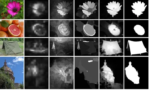
Image LRR [27] ULR [26] SLR [28] SMD(ours) GT
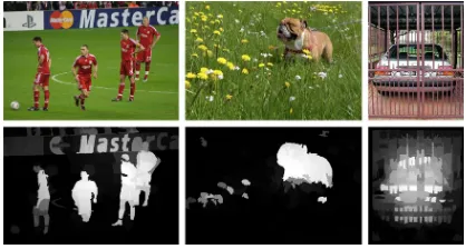
Fig. 1. Typical challenging examples for LR-based salient object de-tection algorithms. The resulting saliency maps of previous solutions (LRR [27], ULR [26] and SLR [28]) are scattered and incomplete, while our algorithm (SMD) overcomes these difficulties and performs close to the ground truth (GT).
function,k·k1is the`1-norm which promotes sparsity, and
the parameterλ >0controls the tradeoff between the two
items.
Though previous LR-based salient object detection algo-rithms ( [26]–[28]) have produced promising results, there still exist several problems:
• Previous studies do not take into account the
inter-correlation between elements in S, and thus ignore
spatial relations, such as spatial contiguity and pattern consistency, between pixels and patches. Algorithms de-signed this way may suffer from two limitations: (1) the foreground pixels or patches in the generated saliency map tend to be scattered, as shown in Fig. 1 (LRR and ULR); and (2) the saliency values may be inconsistent within the same object, causing incompleteness of the detected object, as shown in Fig. 1 (LRR, ULR and SLR).
• According to the LR theory (a.k.a robust PCA) [29], the
decomposition performance of an observation matrix degrades when there is high coherence between the un-derlying low-rank and sparse matrices. Therefore, when the background is cluttered or has similar appearance with the salient objects, it is difficult for previous LR-based methods to separate them, as shown in the last two rows of Fig. 1.
To address these issues, we propose a novel structured
matrix decomposition (SMD) model that treats the (salient) foreground/background separation as a problem of low-rank and structured-sparse matrix decomposition. We en-hance the traditional LR model in Eq. (1) with two important
components. First, we introduce a tree-structured
sparsity-inducing normto constrainS, so that the spatial connectivity and feature similarity of image patches are taken into ac-count in matrix decomposition. This constraint is essentially a hierarchical group sparsity norm over a tree structure,
in which an`∞-norm is employed to enforce within-object
patches to share consistent saliency values. Second, we
integrate a Laplacian regularizationto reduce the coherence
between the low-rank and structured-sparse matrices. The regularizer takes into account the geometrical structure of the image, encourages local similar patches to share similar representation, and eventually separates the foreground objects from the background as much as possible. These
properties enable the proposed SMD model to detect salient objects in jumbled scenes, even when the salient objects have a similar appearance to the background. In addition, SMD enhances object completeness which is sometime hard to achieve by previous solutions.
The main contributions of this work are summarized as follows:
• We develop a novel structured matrix decomposition
model, i.e., SMD, for salient object detection. Compared to the classical LR model used in [26]–[28], SMD not only captures the underlying structure of data, but also better handles the challenges arising from coherence of the low-rank and sparse matrices. To the best of our knowl-edge, this is the first work that explicitly pursues the hierarchical structure of data via structured sparsity in
matrix decomposition. Based on thealternating direction
method(ADM) [31], we derive an effective optimization algorithm to solve the proposed SMD model.
• We present an SMD-based salient object detection
frame-work and evaluate the SMD method on five popular benchmarks involving various scenarios such as single object, multiple objects and complex scenes. Also, we compare our method with 24 state-of-the-art method-s umethod-sing method-six performance metricmethod-s, including the tradi-tional measures, e.g., precision-recall curve and mean
absolute error, and the recently proposed weighted F
-measure [32]. In the experiments, our SMD-based algo-rithm achieves competitive results in comparison with other leading methods.
The remainder of this paper is organized as follows. Sec. 2 reviews existing saliency detection models, especially the LR-based methods. Sec. 3 describes the proposed SMD mod-el and derives the ADM-based solution to the modmod-el. Sec. 4 presents the SMD-based salient object detection method and extends it to integrate high-level priors. Sec. 5 shows the experimental results, including a thorough comparison with recently proposed salient object detection algorithms and detailed analysis of the components in our algorithm. Finally, Sec. 6 concludes the paper.
2
R
ELATEDW
ORKRecent years have witnessed significant advances in saliency detection that includes two major subfields: eye fixation prediction and salient object detection. Recent surveys on eye fixation prediction can be found in [33]–[35], and salient object detection is surveyed in [36], [37]. In this section, we mainly discuss the algorithms belonging to the second subfield, to which our work belongs. But before that, we briefly review some classical early studies that have paved the way to both subfields.
The foundation of most saliency detection algorithm-s can be traced back to the theoriealgorithm-s of center-algorithm-surround difference [38] and multiple feature integration [39]. The most influential model based on the theories is proposed
by Ittiet al.[11], who derive saliency from the difference of
the theories by taking account of local [43], [44], regional [45], and global [46] contrast cues, or by searching for saliency cues in the frequency domain [14], [47].
One of the earliest works onsalient object detectionis [48],
which formulates saliency detection as a binary segmen-tation problem. Recent studies can be broadly categorized as either bottom-up or top-down. Bottom-up models are bio-inspired and only use low-level image features. The frequency tuning method [49] detects saliency by computing color deviation from the mean image color at the pixel level. Later, an improved solution [7] is proposed to highlight salient objects with respect to their contexts in terms of low-level feature distinction and global spatial relations. The global contrast method [12] identifies salient regions by
estimating dissimilarities betweenLabcolor histograms over
all image regions. Saliency filters [50] improve the global contrast method [12] by combining color uniqueness and spatial distribution of image regions. Some other bottom-up techniques such as multi-scale modeling [51] and high-dimensional color transformation [17] have been explored for salient object detection. The effectiveness of other com-plementary cues such as texture [20], depth [52], [53] or surroundedness [54] have also been considered recently.
By contrast, top-down models usually estimate saliency via task-specific learning algorithms or high-level priors.
The method in [48] identifies salient objects using a
condi-tional random field(CRF) on a multi-scale contrast histogram and spatial distribution features. The latent variable model in [55] estimates saliency by jointly learning a CRF and a specific dictionary. Instead of direct training on image features, saliency aggregation [56] trains a CRF on salien-cy maps produced by other methods. The random forest model [57] predicts image saliency by training a regressor on discriminative regional features. Most recently, multiple kernel learning [58] and convolutional neural network [59] techniques have been introduced to learn more robust dis-crimination between salient and non-salient regions.
High-level priors have also been used in top-down mod-els and proved to be effective. For example, a Gaussian fall-off function is frequently recruited to emphasize the center
regions (i.e.,center prior), either directly combined with other
cues [19], [21], [60], or used as a spatial feature in learn-ing [48], [57]. The prior belief that image boundary regions
are more likely to belong to the background (i.e.,background
prior) is also commonly integrated for saliency computation. A representative work is the geodesic saliency [24], which defines boundary regions as terminal nodes when estimat-ing saliency on an image graph. Alternatively, in [61], [62], boundary regions are used as pseudo-background queries and dictionary templates to facilitate detection. Later, a more robust boundary connectivity prior is introduced in [63].
Besides, theobjectness prior, which estimates the likelihood
of a region being a complete object [2], has been employed in some other saliency models [18], [64], [65].
Our study is related to recent methods that consider thesparsity priorin salient object detection. The method in [25] adopts an over-complete dictionary to encode image patches and then feed the coding vector to the LR model to recover salient objects. Later, a supervised method [26] is proposed to leverage feature transformation with the high-level center, color and semantic priors to meet the
low-rank and sparse properties. To better fit the LR model, the segmentation prior derived from the connectivity between regions and image borders is exploited to guide matrix
re-covery [28]. As an extension of the LR model,low-rank
repre-sentation(LRR) [27] introduces a self-representation scheme that reconstructs background regions from the image fea-tures themselves rather than by a dictionary. Multi-feature collaborative enhancement and top-down priors obtained from [66] are incorporated into the multi-task extension.
Difference to related LR-based methods. As an LR-based method, our SMD differs from the previous ones [25]–[28] in several aspects. (1) SMD pursues the low matrix rank in a purely unsupervised way, while [25] and [26] respec-tively resort to supervised sparse representation and feature transformation. The learnt representation or transformation in [25] and [26] is biased toward the training datasets, and therefore suffers from limited adaptability. (2) Our method explicitly encodes information about image structure, i.e., spatial relations and feature similarities of image patches, which are ignored in [25]–[28]. (3) Our method integrates high-level priors into the structured image representation (index tree), while other methods [26], [28] combine such priors by re-weighting the feature.
Discussion with Manifold Ranking (MR) methods. The use of the Laplacian regularization in our method is inspired by, but different from that in the MR algorithm [61]. (1) Our method uses the Laplacian regularization to smooth the feature representation, and to enlarge the difference between foreground objects and background in feature space. By con-trast, MR exploits the regularization to enforce continuous saliency values over neighboring patches. (2) MR is built upon the semi-supervised ranking model [67], and defines saliency of an patch as its relevance to the given querying seeds. By contrast, our method uses the low-rank matrix decomposition framework and is purely unsupervised.
Difference with preliminary work. Some preliminary ideas in this paper appeared in the conference version [68]. Com-pared with [68], the proposed SMD model in this paper is more general, and subsumes the version in [68] as a special case. The new SMD model not only inherits the major advantages of the preliminary model, i.e., it produces a decomposition of an observation matrix into structured parts with respect to image structure, but it is also armed with the new capability to enlarge the separation between salient objects and background in the feature space. The experimental results (Sec. 5) show clearly that the new model is more robust and the resulting saliency maps (Fig. 8) are more visually favorable.
3
S
TRUCTUREDM
ATRIXD
ECOMPOSITIONM
ODEL3.1 Proposed Model
3.1.1 Basic formulation
Given an input imageI, it is first partitioned into N
non-overlapping patchesP = {P1, P2,· · ·, PN}, e.g.,
superpix-els. For each patch Pi, a D-dimension feature vector is
extracted and denoted asfi ∈RD. The ensemble of feature
vectors forms a matrix representation of I, denoted as
F = [f1,f2, . . . ,fN] ∈RD×N. The problem of salient object
detection is to design an effective model to decompose the
2 4 6 8 10 12 14 16 18 20 22 24 0 0.05 0.1 0.15 0.2 0.25 0.3 0.35 0.4
Rank ˆrof Feature Matrix
[image:5.612.313.562.42.143.2]P ro b a b il ity o f O cc u re n ce MSRA10K DUT-OMRON iCoSeg SOD ECSSD
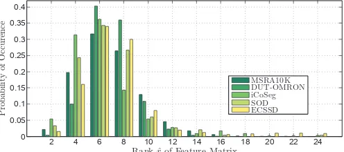
Fig. 2. Rank statistics of feature matrices extracted from image back-ground over five datasets: MSRA10K [48], [69], DUT-OMRON [61], SOD [70], iCoSeg [71] and ECSSD [21].
non-salient background) and a structured distinctive partS
(i.e., salient foreground).
To address the issues discussed in Sec. 1, we propose
a novelstructured matrix decomposition(SMD) model as
fol-lows:
min
L,SΨ(L) +αΩ(S) +βΘ(L,S) s.t. F=L+S, (2)
whereΨ(·)is a low-rank constraint to allow identification of
the intrinsic feature subspace of the redundant background
patches,Ω(·)is a structured sparsity regularization to
cap-ture the spatial and feacap-ture relations of patches inS,Θ(·,·)
is an interactive regularization term to enlarge the distance
between the subspaces drawn fromLand S, and α, β are
positive tradeoff parameters.
3.1.2 Low-rank regularization for image background
Having observed that image patches from the background are often similar and approximately lie in a low-dimensional subspace, we apply low-rank regularization on the
back-ground feature matrix L to pursue its intrinsic structure.
Since directly minimizing a matrix’s rank with affine con-straints is an NP-hard problem [30], we instead adopt the nuclear norm as a convex relaxation, i.e.,
Ψ(L) =rank(L) =kLk∗+ε , (3)
whereεdenotes the relaxation error.
To verify the rationality of the low-rank constraint, we evaluate the rank of feature matrices extracted from image background on five salient object datasets (Fig. 2). Specifical-ly, we first divide each image into a regular grid of patches
of size10×10pixels, excluding those “foreground” patches,
which have over 10% pixels from the annotated salient
objects. Then, each patch is represented by a feature vector encoding color, edge and texture information (as described in Sec. 4.1). Features from the same image are juxtaposed into a matrix to represent the image background. Finally,
we estimate the rank of the feature matrix, denoted by br,
according to [72], [73]:
b
r= arg min
r
RMSRE(r−1)−RMSRE(r)
≤ , (4)
whereRMSRE(r)is theroot mean square reconstruction error
between the original matrix and its rank-r approximation
estimated by the singular value decomposition (SVD), and
is a threshold with value 0.01. Fig. 2 shows the statistics of such estimated ranks of background feature matrices of
the images in the five datasets. It shows that about 90%
of these matrices can be approximated by a matrix with
1
2 3 5 6
4 7 8
1
2 3 5
4 7 8
8 1 1 G 2 1 G 2 3 G 3 1 G 3 3 G 3 4 G 3 5 G
3 5 6
[image:5.612.50.298.45.155.2]4 7 6 1 2 3 2 G (A) (B) 2 2 G 1 1
G
2 1G
2 2G
3 4G
2 3G
3 3 G 3 2 G 3 1G
Fig. 3. The construction of an index tree from an image. (A): The hierarchical segmentation of an input image. The digits are the indexes of patches. (B): An index tree constructed over the indices of image patches{1,2, . . . ,8}. Depth 1 (Root):G1
1={1,2,3,4,5,6,7,8}. Depth
2:G2
1={1,2,3,4},G 2
2 ={5,6},G 2
3={7,8}. Depth 3:G 3
1 ={1,2}, G3
2={3,4},G33={5},G34={6}.
rank no greater than 10. This confirms our intuition that the image background usually lies in a low-dimensional subspace. Therefore, it encourages us to exploit a low-rank regularization to eliminate redundant information and pursue the intrinsic low-dimensional structure.
3.1.3 Structured-sparsity regularization for salient objects
In Eq. (1), the`1-norm regularization treats the columns in
Sindependently and thus ignores spatial structure
informa-tion, which can otherwise be used to improve salient object detection (see Fig. 1). In the following, we introduce a novel tree-structured sparsity-inducing norm to model the spatial contiguity and feature similarity among image patches so as to produce more precise and structurally consistent results.
Before detailing the structured regularization, we first
give the definition of an index tree[74]. An index tree is a
hierarchial structure, such that each node contains a set of indices (e.g., corresponding to the superpixels in our task) and the set is the union of the indices of its children. More
specifically, for an index tree T with depthd over indices
{1,2, . . . , N}, let Gi
j be the j-th node at the i-th level. In
particular, for the root node, we have G1
1 = {1,2, . . . , N}.
The nodes also satisfy two conditions: (1) there is no overlap
between the indices of nodes from the same level, i.e.,Gi
j∩
Gi
k =∅,∀2≤ i≤ dand1 ≤ j < k ≤ni. Here, ni denotes
the total number of nodes at thei-th level. (2) LetGij−10 be
the parent node of a non-root nodeGi
j, thenGij⊆G i−1 j0 and
S
jGij = G i−1
j0 . Fig. 3 shows an example tree with N = 8
indexes, drawn from hierarchical segmentation of an image.
We use an index treeT to encode the spatial relation of
image patchesP. Details of index tree construction are
post-poned to Sec. 4.1. We encode the structurally meaningful tree constraint into a sparsity norm to regularize the matrix decomposition. In this way, we get a general tree-structured sparsity regularization as
Ω(S) =
d X i=1 ni X j=1
vijkSGi
jkp, (5)
wherevi
j ≥0is the weight for the nodeGij,SGi
j ∈R D×|Gij|
(|·| denotes set cardinality) is the sub-matrix of S
corre-sponding to the node Gi
j, and k·kp is the `p-norm1, 1 ≤
p≤ ∞. In essence,Ω(·)is a weighted group sparsity norm
defined over a tree structure. It induces the patches within
1. For a matrixA= (aij)∈Rm×n, kAkp= ( m P i=1 n P j=1
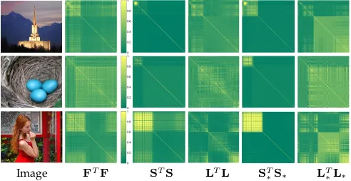
Image FTF STS LTL ST
[image:6.612.50.296.43.170.2]∗S∗ LT∗L∗ Fig. 4. The pairwise similarity matrices of feature vectors before and after imposing Laplacian regularization. The upper-left block in the matri-ces represents the similarities of foreground patches, while the bottom-right block indicates the similarities of background patches. Matrices with subscript ‘∗’ are the results after imposing Laplacian regularization.
the same group to share a similar representation, and also represents the subordinate or coordinate relations between groups. To enforce the patches from the same group to have
identical saliency values, we impose the`∞-norm onSGi
j,
i.e.,p =∞. It uses the maximum saliency value of patches
within the groupGij to decide whether the group is salient
or not [75].
3.1.4 Laplacian regularization
When decomposing the feature matrix F into a low-rank
part L plus a structured-sparse part S, we also hope to
enlarge the distance between the subspaces induced by
L and S, so as to make it easier to separate the salient
object from the background. To this end, we introduce a Laplacian regularization based on the local invariance assumption [76]: if two adjacent image patches are similar with respect to their features, their representations should be close to each other in the subspace, and vise versa. Thus motivated, we define the regularization as
Θ(L,S) = 1
2 N
X
i,j=1
ksi−sjk22wi,j= Tr(SMFST), (6)
wheresidenotes thei-th column ofS,wi,jis the(i, j)-th
en-try of an affinity matrixW= (wi,j)∈RN×Nand represents
the feature similarity of patches (Pi, Pj),Tr(·) denotes the
trace of a matrix, and MF ∈RN×N is a Laplacian matrix.
Specifically, the affinity matrixWis defined as
wi,j =
(
exp − kfi−fjk2
2σ2
, if (Pi, Pj)∈V,
0, otherwise, (7)
whereV denotes the set of adjacent patch pairs which are
either neighbors (first-order) or “neighbors of neighbors”
(second-order reachable) on the image. The(i, j)-th entry of
the Laplacian matrixMFis
(MF)i,j=
−wi,j, if i6=j ,
P
j6=iwi,j, otherwise. (8)
It is interesting to find that the Laplacian regularization
in Eq. (6) is explicitly related with F and S, and can
be transferred to be related with L and S according to
Θ(F,S) = Θ(L+S,S) = Θ(L,S). Essentially, the
Lapla-cian regularization increases the distance between feature
subspaces by smoothing the vectors in S according to
the local neighborhood derived from the feature matrix
Algorithm 1ADM-SMD.
Input: Feature matrix F, parameters α, β, index tree T =
{Gi
j}and tree node weightvij(default as 1).
Output: LandS.
1: Initialize L0=0, S0=0, H0=0, Y0
1=0, Y02=0, µ0=0.1,
µmax= 1010,ρ= 1.1, andk= 0.
2: Whilenot converged do
3: Lk+1 = arg min
L
L(L,Sk,Hk,Yk
1,Y2k, µk)
4: Hk+1= arg min
H
L(Lk+1,Sk,H,Y1k,Yk2, µk)
5: Sk+1 = arg min
S
L(Lk+1,S,Hk+1,Yk
1,Y2k, µk)
6: Yk1+1=Yk
1+µk(F−Lk+1−Sk+1)
7: Yk2+1=Yk
2+µk(Sk+1−Hk+1)
8: µk+1= min (ρµk, µ
max)
9: k=k+ 1
10: End While
11: Return LkandSk.
F. It encourages patches within the same semantic region
[image:6.612.315.563.92.251.2]to share similar or identical representation, and patches from heterogeneous regions to have different representation.
Fig. 4 shows the pairwise similarity of the elements inLand
Sbefore and after imposing the Laplacian regularization. It
shows that a more distinct block affinity matrix is produced by using the regularization.
3.2 Optimization
Considering the balance between efficiency and accuracy
in practice, we resort to thealternating direction method
(AD-M) [31] to solve the convex problem defined in Eq. (2). We
first introduce an auxiliary variableHto make the objective
function separable, i.e., Eq. (2) becomes
min
L,S kLk∗+α d
X
i=1 ni
X
j=1
vjikSGi
jkp+βTr(HMFH T)
s.t. F=L+S, S=H.
(9)
Then, the problem (9) can be solved with ADM, which
minimizes the following augmented Lagrangian functionL:
L(L,S,H,Y1,Y2, µ) =kLk∗
+α
d
X
i=1 ni
X
j=1
vijkSGi
jkp+βTr(HMFH T)
+ Tr(Y1T(F−L−S)) + Tr(YT2(S−H))
+µ
2 kF−L−Sk
2
F +kS−Hk 2 F
,
(10)
where Y1 and Y2 are the Lagrange multipliers, and µ >
0 controls the penalty for violating the linear constraints.
To solve Eq. (10), we search for the optimal L, S and H
iteratively, and in each iteration the three components are updated alternately. We outline the optimization procedure in Algorithm 1 and call it ADM-SMD. In the following, we provide the details for each iteration.
UpdatingL: When SandHare fixed, the update Lk+1 at
problem:
Lk+1= arg min
L
L(L,Sk,Hk,Y1k,Yk2, µk)
= arg min
L
kLk∗+ Tr((Yk1)T(F−L−Sk))
+µ
k
2 kF−L−S
kk2 F
= arg min
L
τkLk∗+
1
2kL−XLk
2 F ,
(11)
whereτ = 1/µkandXL=F−Sk+Yk1/µk. The solution to
Eq. (11) can be derived as
Lk+1=UTτ[Σ]VT,where (U,Σ,VT) =SVD(XL). (12)
Note thatΣis the singular value matrix ofXL. The operator
Tτ[·]is thesingular value thresholding(SVT) [77] defined by
element-wiseτ thresholding ofΣ. Specifically, letσibe the
i-th diagonal element ofΣ, thenTτ[Σ]is a diagonal matrix
defined as
Tτ[Σ] = diag({(σi−τ)+}), (13)
wherea+is the positive part ofa, namely,a+= max(0, a).
UpdatingH: WhenLandSare fixed, to updateHk+1, we derive from Eq. (10) the following problem:
Hk+1= arg min
H
L(Lk+1,Sk,H,Yk1,Yk2, µk)
= arg min
H
βTr(HMFHT)+Tr((Y2k)T(Sk−H))
+µ
k
2 kS
k−Hk2 F .
(14)
Taking derivative of the objective function in Eq. (14) (the detailed derivation is presented in Appendix A), we have
Hk+1 = (µkSk+Yk2)(2βMF+µkI)−1. (15)
UpdatingS: To updateSk+1with fixedLandH, we get the
following tree-structured sparsity optimization problem:
Sk+1= arg min
S
L(Lk+1,S,Hk+1,Yk1,Y2k, µk)
= arg min
S
α
d
X
i=1 ni
X
j=1
vijkSGi jkp
+Tr((Yk
1)T(F−Lk+1−S))+Tr((Yk2)T(S−Hk+1))
+µ
k
2 (kF−L
k+1−Sk2
F+kS−Hk+1k2F)
= arg min
S
λ
d
X
i=1 ni
X
j=1
vjikSGi jkp+
1
2kS−XSk
2 F ,
(16)
where λ = α/(2µk) and XS = (F−Lk+1+Hk+1+ (Yk1 −
Yk
2)/µk)/2. The above problem can be solved by the
hierar-chical proximal operator [78], which computes a particular sequence of residuals obtained by projecting a matrix onto
the unit ball of dual`p-norm. The detailed procedure when
using`∞-norm is presented in Algorithm 2.
4
SMD-
BASEDS
ALIENTO
BJECTD
ETECTIONIn this section, we describe our salient object detection algo-rithm that uses the proposed SMD model. Our algoalgo-rithm includes two major parts: the first one focuses on low-level features, while the second one incorporates high-low-level prior knowledge. Fig. 5 shows the framework of SMD-based salient object detection.
Algorithm 2Solving the tree-structured sparsity.
Input: The index treeT with nodesGi
j (i = 1,2, ..., d;j = 1,2, ..., ni), weightvij ≥0(default as 1), the matrixXS,
parametersα, and setλ=α/(2µk).
1: SetS=XS
2: Fori=dto1 do
3: Forj= 1toni do
4: SkG+1i j
=
SGi
j
1−λv
i j
SGi
j
1
SGi j, if
SGi
j
1> λv i j
0, otherwise
5: End For
6: End For
7: Return Sk+1
4.1 Low-level Salient Object Detection
Our framework for low-level salient object detection consist-s of four consist-stepconsist-s: image abconsist-straction, index tree conconsist-struction, matrix decomposition and saliency assignment.
Step 1: Image Abstraction. In this step, an input im-age is partitioned into compact and perceptually homoge-neous elements. Following [26], we first extract the low-level features, including RGB color, steerable pyramids [79] and Gabor filter [80], to construct a 53-dimension feature
representation. Then, we perform the simple linear iterative
clustering(SLIC) algorithm [81] to over-segment the image
into N atom patches (superpixels) P = {P1, P2,· · ·, PN}.
Each patch Pi is represented by a feature vector fi, and
all these feature vectors form the feature matrix as F =
[f1,f2, . . . ,fN]∈RD×N(hereD= 53).
Step 2: Tree Construction.On top ofP, an index treeT is constructed to encode structure information via hierarchical segmentation. To this end, we first compute the affinity of every adjacent patch pair using Eq. (7). Then, we apply a graph-based image segmentation algorithm [82] to merge spatially neighboring patches according to their affinity. The algorithm produces a sequence of granularity-increasing segmentations. In each granularity layer, the segments cor-respond to the nodes at the corcor-responding layer in the index tree. Specifically, the granularity is controlled by a affinity
thresholdT. Finally, we obtain a hierarchical fine-to-coarse
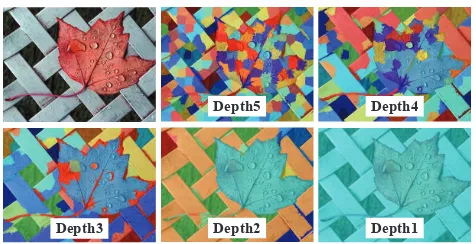
segmentation of the input image. Fig. 6 shows a visualized example of hierarchical segmentation, corresponding to a five-layer index tree structure.
Step 3: Matrix Decomposition. When both the feature
matrix F and the index tree T are ready, we apply the
proposed SMD model, formulated as Eq. (2) with `∞
-norm, to decomposeFinto a low-rank componentLand a
structured-sparse componentS. As shown in Step 3 of Fig. 5,
after jointly imposing the structured-sparsity and Laplacian
regularization, the input feature matrix F is decomposed
into structured componentsLandS.
Step 4: Saliency Assignment. After decomposing F, we transfer the results from the feature domain to the spatial domain for saliency estimation. Based on the structured
matrix S, we define a straightforward saliency estimation
functionSal(·)of each patch inP:
Sal(Pi) =ksik1, (17)
where si represents thei-th column of S. A large Sal(Pi)
Original Image
Saliency Map A Structured Index Tree
Over-segmentation
i
f
Low Rank Part (L) Structured Sparse Part (S)
Gi j
Feature Extraction Feature Matrix (F) High-level Prior
Map
Location Prior
Color Prior
Background Prior
1 1
G
2 1
G 2
j
G
1
d
G
2 2
n
G
1 d d n
G- d d n
G
'
j d
G
2
d
G
i
[image:8.612.55.557.43.209.2]P
Fig. 5. Framework of the SMD model for salient object detection.
Depth5 Depth4
Depth3 Depth2 Depth1
Fig. 6. Illustration of index tree construction based on the graph-based clustering. Each image indicates one layer in the index tree, while each patch represents one node.
After merging all patches together and performing context-based propagation (section 3.2 in [62]), we get the final saliency map of the input image.
4.2 Integrate High-level Priors
We further extend the proposed SMD-based saliency de-tection to integrate high-level priors. Inspired by the work of Shen and Wu [26], we fuse three types of priors, i.e. location, color and background priors, to generate a high-level prior map. Specifically, the location prior is generated by a Gaussian distribution based on the distances of the pixels from the image center. The color prior used here is the same as [26], which measures human eye sensitivity to red and yellow color. The background prior calculates the probabilities of image regions connected to image bound-aries [63]. These three priors are finally multiplied together to produce the high-level prior map (see Fig. 5).
For each patch Pi ∈ P, its high-level prior, πi ∈ [0,1],
indicates the likelihood that Pi belongs to a salient object
based on high-level information. This prior is encoded into the SMD by weighting each component in the tree-structured sparsity-inducing norm differently. In particular, we definevijas
vij= 1−max {πk:k∈Gij}
. (18)
Eq. (18) essentially boosts the saliency value of nodes with high prior values by associating them with small penalties
vi
j. This way, the high-level prior knowledge is seamlessly
encoded into the SMD model to guide the matrix decompo-sition and enhance the saliency detection. It is worth noting that if we fixvi
j= 1for each nodeGij, the proposed model
[image:8.612.54.292.220.342.2]is degraded to the pure low-level saliency detection model.
TABLE 1
Summary of the benchmark datasets.
Name Size Characteristics MSRA10K
[69] 10,000(imgs) single object, collected from MSRA [48],simple background, high contrast
DUT-OMRON [61] 5,168 single object, relatively complexbackground, more challenging iCoSeg [71] 643 multiple objects, various number of
objects with different sizes SOD [70] 300 multiple objects, various size and
location of objects, complex background ECSSD [50] 1,000 structurally complex natural images,
various object categories
5
E
XPERIMENTTo fully evaluate our algorithm, we conduct a series of ex-periments using five benchmark datasets involving various scenarios and include 24 recent solutions for comparison.
5.1 Experimental Setup
5.1.1 Datasets
We use five popular benchmark datasets to cover different scenarios. In particular, we use MSRA10K [69] and DUT-OMRON [61] for images with a single salient object, i-CoSeg [71] and SOD [70] for cases with multiple salient objects, and ECSSD [21] for images with complex scenes. The size and detailed characteristic of these benchmark datasets are presented in Tab. 1.
5.1.2 Salient object detection algorithms
The proposed salient object detection algorithm is compared with 24 state-of-the-art solutions, including three LR-based methods (ULR [26], LRR [27] and SLR [28]), four methods ranked the highest according to the survey in [36] (SVO [18],
CA [7], CB [19] and RC [12]), and 17 recently developed
prominent methods (RBD [63], HCT [17], DSR [62], MC [83], GC [23], DRFI [57], PCA [22], HS [21], TD [20], MR [61], GS [24], SF [50], SS [15], SEG [13], FT [49], LC [16] and SR [14]). Tab. 2 summarizes all the algorithms involved in our experiments.
5.1.3 Parameter settings
The parameters in the implementation of the proposed SMD detector are set as follows. In image abstraction, we set the
number of patchesN to 200. In tree construction, we set the
affinity thresholds asT = [100,400,2000], producing three
TABLE 2
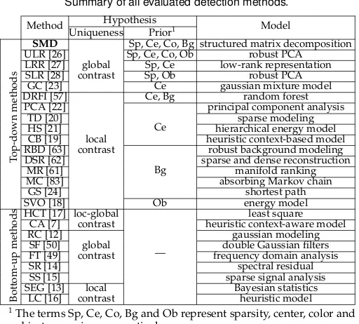
Summary of all evaluated detection methods.
Method Hypothesis Model Uniqueness Prior1
T
op-down
methods
SMD Sp, Ce, Co, Bg structured matrix decomposition ULR [26] Sp, Ce, Co, Ob robust PCA
LRR [27] global Sp, Ce low-rank representation SLR [28] contrast Sp, Ob robust PCA
GC [23] Ce gaussian mixture model DRFI [57] Ce, Bg random forest PCA [22]
Ce
principal component analysis TD [20] sparse modeling HS [21] hierarchical energy model CB [19] local heuristic context-based model RBD [63] contrast
Bg
robust background modeling DSR [62] sparse and dense reconstruction
MR [61] manifold ranking MC [83] absorbing Markov chain
GS [24] shortest path SVO [18] Ob energy model
Bottom-up
methods
HCT [17] loc-global
—
least square CA [7] contrast heuristic context-aware model RC [12] gaussian modeling
SF [50] global double Gaussian filters FT [49] contrast frequency domain analysis SR [14] spectral residual SS [15] sparse signal analysis SEG [13] local Bayesian statistics
LC [16] contrast heuristic model
1The terms Sp, Ce, Co, Bg and Ob represent sparsity, center, color and
objectness priors, respectively.
set the bandwidth parameter δ2 to 0.05, and the model
parametersαandβto0.35and1.1respectively.
To retain a fair comparison with competing methods, we fix the parameters of our model for all the experi-ments. It is worth noting that by tuning the parameters on the datasets, our model still has some potential to be improved, as presented in Appendix B. For other algo-rithms in our comparison, we use the source or binary codes provided by the authors with default parameters. The source code of our method and all experimental results
are publicly available at http://www.dabi.temple.edu/∼hbling/
SMD/SMDSaliency.html. Our code is implemented in mixed
C++ and Matlab, and its average runtime is1.217 seconds
per image on MSRA10K using a PC of 3.4 GHz and 4GB RAM, with only a single thread used.
5.1.4 Evaluation metrics
For comprehensive evaluation, we use seven metrics
includ-ing the precision-recall (PR) curve, theF-measure curve, the
receiver operating characteristic (ROC) curve, area under the ROC curve (AUC), mean absolute error (MAE),
overlap-ping ratio (OR) and the weightedF-measure (WF) score.
Precision is defined as the percentage of salient pixels correctly assigned, while recall is the ratio of correctly
detected salient pixels to all true salient pixels.F-measure
is a weighted harmonic mean of precision (P) and recall
(R):Fβ = (1 +β2)P ·R/(β2P+R), whereβ2is set to 0.3 to
stress precision more than recall [49]. The PR andF-measure
curves are created by varying the saliency threshold that determines whether a pixel belongs to the salient object. The ROC curve is generated from true positive rates and false positive rates which are obtained when we calculate the PR curve.
Although commonly used, the above metrics ignore the effects of correct assignment of non-salient pixels and the importance of complete detection. We therefore introduce the MAE and OR metrics to address these issues. Given a
continuous saliency mapSand the binary ground truthG,
MAE is defined as the mean absolute difference betweenS
andG:MAE = mean(|S−G|)[50]. OR is defined as the
over-lapping ratio between the segmented object mask S0 and
ground truthG:OR =|S0∩G|/|S∪G|, whereS0is obtained
by binarizingS using an adaptive threshold, i.e., twice the
mean values ofS as in [51]. Finally, we adopt the recently
proposed weightedF-measure (WF) metric [32], which is a
weighted version of the traditional F-measure. It amends
the interpolation, dependency and equal importance flaws of currently-used measures.
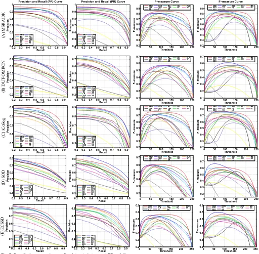
5.2 Comparison with State-of-the-Arts
The proposed SMD algorithm is evaluated on the five benchmark datasets and compared with 24 recently pro-posed algorithms. The results are summarized in Tab. 3 and Fig. 7. Besides, Fig. 8 shows some qualitative comparisons.
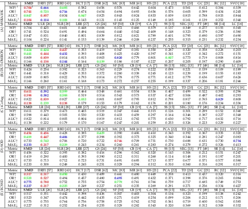
The results show that, in most cases, SMD ranks first or second on the five benchmark datasets across different criteria. It is worth noting that, although DRFI [57] is the best performing method, it is a supervised one requiring a large amount of training. In contrast, our method is an unsupervised one, which skips the training process and therefore enjoys more flexibility.
5.2.1 Results on single-object images
The test on images with a single object is conducted on the MSRA10K [69] and DUT-OMRON [61] datasets. The PR and
F-measure curves are shown in Fig. 7(A and B), and the WF,
OR, AUC and MAE scores in Tab. 3(A and B).
On MSRA10K (Tab. 3(A)), SMD achieves the best per-formance in terms of WF, OR and MAE, while DRFI [57] obtains the best AUC score. In the PR curves (Fig. 7(A)), DRFI [57] and SMD are the best two among those
competi-tive methods. In theF-measure curves, SMD is superior, as
it achieves relatively good results over a large range. On DUT-OMRON (Tab. 3(B)), all the methods perform worse than on MSRA10K due to the large diversity and complexity of DUT-OMRON. SMD performs the second best in terms of WF and OR, with a very minor margin (0.003) to the best results. The best MAE and AUC scores are achieved by DRFI [57]. This is because DRFI takes advantage of multi-level saliency maps fusion to improve its robustness. The fusion strategy is effective and general, as discussed in Appendix C. In the PR curves (Fig. 7(B)), the precision of SMD is less impressive at low recall rates, but it
is competitive at the high recall rates. In terms ofF-measure,
SMD obtains relatively superior performance, especially when segmenting saliency maps with high thresholds.
5.2.2 Results on multiple-object images
Experiments on images with multiple salient objects are
conducted on iCoSeg [71] and SOD [70]. The PR and F
-measure curves are shown in Fig. 7(C and D), and the WF, OR, AUC and MAE scores in Tab. 3(C and D).
On iCoSeg (Tab. 3(C)), SMD achieves the best perfor-mance in terms of WF, OR and MAE. The AUC score of SMD is a little lower than the best, achieved by DRFI [57].
Fig. 7(C) shows that the PR andF-measure curves of SMD
are superior or comparable to other methods. In particular,
SMD’sF-measure remains high over a wide range,
indicat-ing its insensitivity to the selection of a threshold.
TABLE 3
Results on five datasets in terms of WF, AUC, OR and MAE.
(A)
MSRA10K
Metric SMD DRFI [57] RBD [63] HCT [17] DSR [62] MC [83] MR [61] HS [21] PCA [22] TD [20] GC [23] RC [12] SVO [18] WF↑1 0.7042 0.666 0.685 0.582 0.656 0.576 0.642 0.604 0.473 0.561 0.612 0.384 0.339
OR↑ 0.741 0.723 0.716 0.674 0.654 0.694 0.693 0.656 0.576 0.605 0.599 0.434 0.245
AUC↑ 0.847 0.857 0.834 0.847 0.825 0.843 0.824 0.833 0.839 0.815 0.788 0.833 0.844 MAE↓1 0.104 0.114 0.108 0.143 0.121 0.145 0.125 0.149 0.185 0.161 0.139 0.252 0.340 Metric SMD ULR [26] SLR [28] LRR [27] GS [24] SF [50] CB [19] CA [7] SS [15] SEG [13] FT [49] SR [14] LC [16]
WF↑ 0.704 0.425 0.601 0.448 0.606 0.372 0.466 0.379 0.137 0.349 0.277 0.155 0.345 OR↑ 0.741 0.524 0.691 0.494 0.664 0.440 0.542 0.409 0.148 0.323 0.379 0.256 0.380 AUC↑ 0.847 0.831 0.840 0.801 0.839 0.812 0.821 0.789 0.601 0.795 0.690 0.597 0.690 MAE↓ 0.104 0.224 0.141 0.153 0.139 0.246 0.208 0.237 0.255 0.315 0.231 0.232 0.234
(B)
DUT
-OMRON
Metric SMD DRFI [57] RBD [63] HCT [17] DSR [62] MC [83] MR [61] HS [21] PCA [22] TD [20] GC [23] RC [12] SVO [18] WF↑ 0.424 0.424 0.427 0.353 0.419 0.347 0.381 0.350 0.287 0.320 0.358 0.228 0.203 OR↑ 0.441 0.444 0.432 0.393 0.408 0.425 0.420 0.397 0.341 0.337 0.342 0.272 0.151 AUC↑ 0.809 0.839 0.814 0.815 0.803 0.820 0.779 0.801 0.827 0.773 0.719 0.808 0.816 MAE↓ 0.166 0.138 0.144 0.164 0.139 0.186 0.187 0.227 0.207 0.205 0.197 0.290 0.409 Metric SMD ULR [26] SLR [28] LRR [27] GS [24] SF [50] CB [19] CA [7] SS [15] SEG [13] FT [49] SR [14] LC [16]
WF↑ 0.424 0.254 0.392 0.323 0.363 0.229 0.274 0.222 0.098 0.221 0.159 0.109 0.189 OR↑ 0.441 0.318 0.429 0.353 0.372 0.280 0.338 0.245 0.123 0.239 0.199 0.155 0.183 AUC↑ 0.809 0.805 0.822 0.793 0.814 0.778 0.775 0.771 0.612 0.779 0.636 0.607 0.626 MAE↓ 0.166 0.260 0.161 0.168 0.173 0.272 0.257 0.255 0.199 0.337 0.206 0.181 0.246
(C)
iCoSeg
Metric SMD DRFI [57] RBD [63] HCT [17] DSR [62] MC [83] MR [61] HS [21] PCA [22] TD [20] GC [23] RC [12] SVO [18]
WF↑ 0.611 0.592 0.599 0.464 0.548 0.461 0.554 0.536 0.407 0.499 0.522 0.395 0.296
OR↑ 0.598 0.582 0.588 0.519 0.514 0.543 0.573 0.537 0.427 0.506 0.487 0.402 0.293
AUC↑ 0.822 0.839 0.827 0.833 0.801 0.807 0.795 0.812 0.798 0.817 0.765 0.829 0.808
MAE↓ 0.138 0.139 0.138 0.179 0.153 0.179 0.162 0.176 0.201 0.180 0.176 0.234 0.336
Metric SMD LR [26] SLR [28] LRR [27] GS [24] SF [50] CB [19] CA [7] SS [15] SEG [13] FT [49] SR [14] LC [16] WF↑ 0.611 0.379 0.473 0.465 0.519 0.347 0.441 0.315 0.126 0.301 0.289 0.152 0.340 OR↑ 0.598 0.443 0.505 0.530 0.520 0.433 0.459 0.297 0.164 0.346 0.387 0.227 0.348 AUC↑ 0.822 0.814 0.805 0.804 0.819 0.812 0.782 0.775 0.630 0.792 0.717 0.632 0.716 MAE↓ 0.138 0.222 0.179 0.170 0.167 0.247 0.201 0.259 0.253 0.326 0.223 0.229 0.227
(D)
SOD
Metric SMD DRFI [57] RBD [63] HCT [17] DSR [62] MC [83] MR [61] HS [21] PCA [22] TD [20] GC [23] RC [12] SVO [18]
WF↑ 0.456 0.456 0.428 0.385 0.429 0.390 0.406 0.410 0.343 0.392 0.367 0.335 0.320
OR↑ 0.419 0.447 0.406 0.377 0.398 0.392 0.373 0.325 0.340 0.344 0.281 0.247 0.083 AUC↑ 0.733 0.742 0.706 0.720 0.722 0.746 0.709 0.731 0.730 0.688 0.631 0.730 0.734
MAE↓ 0.233 0.217 0.229 0.243 0.234 0.260 0.261 0.283 0.274 0.279 0.272 0.326 0.413
Metric SMD LR [26] SLR [28] LRR [27] GS [24] SF [50] CB [19] CA [7] SS [15] SEG [13] FT [49] SR [14] LC [16] WF↑ 0.456 0.322 0.395 0.382 0.416 0.296 0.362 0.320 0.143 0.306 0.212 0.151 0.247 OR↑ 0.419 0.290 0.400 0.393 0.390 0.212 0.311 0.268 0.114 0.148 0.191 0.197 0.201 AUC↑ 0.733 0.713 0.712 0.723 0.731 0.691 0.685 0.713 0.577 0.677 0.571 0.577 0.580 MAE↓ 0.233 0.308 0.248 0.245 0.251 0.329 0.294 0.312 0.310 0.360 0.316 0.291 0.317
(E)
ECSSD
Metric SMD DRFI [57] RBD [63] HCT [17] DSR [62] MC [83] MR [61] HS [21] PCA [22] TD [20] GC [23] RC [12] SVO [18]
WF↑ 0.517 0.517 0.490 0.430 0.489 0.441 0.480 0.449 0.358 0.413 0.437 0.320 0.316
OR↑ 0.523 0.527 0.494 0.457 0.480 0.495 0.491 0.432 0.371 0.398 0.376 0.265 0.084
AUC↑ 0.775 0.780 0.752 0.755 0.754 0.779 0.761 0.766 0.759 0.717 0.685 0.749 0.753
MAE↓ 0.227 0.217 0.225 0.249 0.227 0.251 0.235 0.269 0.291 0.271 0.256 0.334 0.427
Metric SMD ULR [26] SLR [28] LRR [27] GS [24] SF [50] CB [19] CA [7] SS [15] SEG [13] FT [49] SR [14] LC [16] WF↑ 0.517 0.351 0.442 0.398 0.436 0.307 0.403 0.304 0.134 0.323 0.199 0.138 0.242 OR↑ 0.523 0.347 0.474 0.442 0.435 0.271 0.419 0.254 0.099 0.206 0.212 0.171 0.206 AUC↑ 0.775 0.755 0.764 0.756 0.758 0.725 0.762 0.702 0.561 0.719 0.600 0.562 0.585 MAE↓ 0.227 0.312 0.252 0.254 0.255 0.329 0.282 0.343 0.320 0.369 0.312 0.308 0.332
1The up-arrow↑indicates the larger value achieved, the better performance is, while the down-arrow↓indicates the smaller, the better. 2The best three results are highlighted withred,greenandbluefonts, respectively.
is slightly lower than that of DRFI [57], but better than the
others. In theF-measure curves, SMD performs the best at
higher threshold ranges, while DRFI performs the best at lower ranges. Both are consistently superior to the others.
5.2.3 Results on complex scene images
Our last comparison with the competing methods is con-ducted on ECSSD [21], which is known to involve complex scenes. As reported in Tab. 3(E), SMD obtains the best performance in terms of WF, the second or third best in OR, AUC and MAE. According to Fig. 7(E), the PR curve of SMD is the second best among those methods, while the
area under the F-measure curve is the best. These results
validate SMD’s strong potential in handling images with complex scenes.
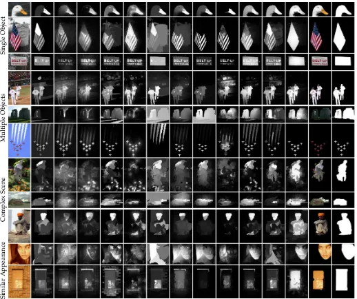
5.2.4 Visual comparison
Fig. 8 shows some visual comparisons of the best methods in the experiments. For single-object images, SMD accurately extracts the entire salient object with few scattered patches, and assigns nearly uniform saliency values to all patches
within the salient objects. For images with multiple objects, some methods (e.g., SLR [28], ULR [26] and MR [61]) miss detecting parts of the objects, while some (e.g., HS [21] and HCT [17]) incorrectly include background regions into detection results. By contrast, SMD pops out all the salient objects successfully. For the images with complex scenes, most methods fail to identify the salient objects, while SMD locates them with decent accuracy. Finally, for the images whose foreground and background share similar appear-ance, SMD successfully separates the salient objects from the background, while other methods often fail. These results illustrate the robustness of the SMD algorithm, and confirm the effectiveness of the proposed structural constraints in separating the coherent low-rank and sparse subspaces.
5.3 Experimental Analysis of the Proposed Method
5.3.1 Analysis of components in the proposed model
0.2 0.3 0.4 0.5 0.6 0.7 0.8 0.9 0.4 0.5 0.6 0.7 0.8 0.9 1 Recall Precision
Precision and Recall (PR) Curve
SMD DSR MC HS PCA ULR SLR LRR RC SF CA FT SR (A) MSRA10K
0.2 0.3 0.4 0.5 0.6 0.7 0.8 0.9 0.4 0.5 0.6 0.7 0.8 0.9 1 Recall Precision
Precision and Recall (PR) Curve
SMD DRFI RBD HCT MR SVO TD GS CB GC SEG SS LC
0 50 100 150 200 250 0.2 0.3 0.4 0.5 0.6 0.7 0.8 0.9 Threshold F−measure F−measure Curve
SMD DSR MC HS PCA ULR SLR LRR RC SF CA FT SR
0 50 100 150 200 250 0.2 0.3 0.4 0.5 0.6 0.7 0.8 0.9 Threshold F−measure F−measure Curve
SMD DRFI RBD HCT MR SVO TD GS CB GC SEG SS LC
0.2 0.3 0.4 0.5 0.6 0.7 0.8 0.9 0.2 0.3 0.4 0.5 0.6 0.7 Recall Precision SMD DSR MC HS PCA ULR SLR LRR RC SF CA FT SR (B) DUT -OMRON
0.2 0.3 0.4 0.5 0.6 0.7 0.8 0.9 0.2 0.3 0.4 0.5 0.6 0.7 Recall Precision SMD DRFI RBD HCT MR SVO TD GS CB GC SEG SS LC
0 50 100 150 200 250 0.1 0.2 0.3 0.4 0.5 0.6 0.7 Threshold F−measure
SMD DSR MC HS PCA ULR SLR LRR RC SF CA FT SR
0 50 100 150 200 250 0.1 0.2 0.3 0.4 0.5 0.6 0.7 Threshold F−measure
SMD DRFI RBD HCT MR SVO TD GS CB GC SEG SS LC
0.2 0.3 0.4 0.5 0.6 0.7 0.8 0.9 0.5 0.6 0.7 0.8 0.9 Recall Precision SMD DSR MC HS PCA ULR SLR LRR RC SF CA FT SR (C) iCoSeg
0.2 0.3 0.4 0.5 0.6 0.7 0.8 0.9 0.5 0.6 0.7 0.8 0.9 Recall Precision SMD DRFI RBD HCT MR SVO TD GS CB GC SEG SS LC
0 50 100 150 200 250 0.2 0.3 0.4 0.5 0.6 0.7 0.8 Threshold F−measure
SMD DSR MC HS PCA ULR SLR LRR RC SF CA FT SR
0 50 100 150 200 250 0.2 0.3 0.4 0.5 0.6 0.7 0.8 Threshold F−measure
SMD DRFI RBD HCT MR SVO TD GS CB GC SEG SS LC
0.2 0.3 0.4 0.5 0.6 0.7 0.8 0.9 0.3 0.4 0.5 0.6 0.7 0.8 Recall Precision SMD DSR MC HS PCA ULR SLR LRR RC SF CA FT SR (D) SOD
0.2 0.3 0.4 0.5 0.6 0.7 0.8 0.9 0.3 0.4 0.5 0.6 0.7 0.8 Recall Precision SMD DRFI RBD HCT MR SVO TD GS CB GC SEG SS LC
0 50 100 150 200 250 0.2 0.3 0.4 0.5 0.6 0.7 Threshold F−measure
SMD DSR MC HS PCA ULR SLR LRR RC SF CA FT SR
0 50 100 150 200 250 0.2 0.3 0.4 0.5 0.6 0.7 Threshold F−measure
SMD DRFI RBD HCT MR SVO TD GS CB GC SEG SS LC
0.2 0.3 0.4 0.5 0.6 0.7 0.8 0.9 0.3 0.4 0.5 0.6 0.7 0.8 Recall Precision SMD DSR MC HS PCA ULR SLR LRR RC SF CA FT SR (E) ECSSD
0.2 0.3 0.4 0.5 0.6 0.7 0.8 0.9 0.3 0.4 0.5 0.6 0.7 0.8 Recall Precision SMD DRFI RBD HCT MR SVO TD GS CB GC SEG SS LC
0 50 100 150 200 250 0.2 0.3 0.4 0.5 0.6 0.7 0.8 Threshold F−measure
SMD DSR MC HS PCA ULR SLR LRR RC SF CA FT SR
0 50 100 150 200 250 0.2 0.3 0.4 0.5 0.6 0.7 0.8 Threshold F−measure
SMD DRFI RBD HCT MR SVO TD GS CB GC SEG SS LC
Fig. 7. Quantitative comparison on five datasets in terms of PR andF-measure curves.
corresponds to an objective function listed in Tab. 4, and parameters for each model are tuned separately to obtain optimal results. Furthermore, only low-level features are used to avoid the influence of high-level prior knowledge.
The quantitative results are shown in Fig. 9(left and mid-dle), leading to the following observations. (1) By comparing
LR-`1 with LR-Tree1, we see that encoding tree-structure
information gives in average improvement of4.69%
[image:11.612.46.558.45.547.2](preci-sion) and2.76%(true positive rate) over the plain`1-norm.
TABLE 4
The objective function of different models related to SMD.
Model Objective Function
LR-`1 minL,SkLk∗+αkSk1 LR-Tree1 minL,SkLk∗+αPG∈TkSGk1 LR-Tree∞ minL,SkLk∗+αPG∈TkSGk∞
SMD minL,SkLk∗+αPG∈TkSGk∞+βTr(SMFST)
(2) The `∞-norm embedding in the structured sparsity
s-lightly improves the`1-norm (comparing LR-Tree1and
LR-Tree∞). (3) The use of the Laplacian regularization
signif-icantly improves the LR-Tree∞ model. These observations
indicate that the introduced regularizers are effective and complementary, and, when combined together, lead to ex-cellent performance as reported in the previous subsection.
We further analyze the underlying reasons for the above observed improvements by comparing the saliency maps. As shown in Fig. 11, we observe that: (1) The salient regions
identified by LR-Tree1 tend to be connected, whereas the
regions identified by LR-`1tend to be scattered. This shows
that the tree-structured constraint guides matrix decom-position along a structurally meaningful direction. (2) The
LR-Tree∞ model produces smoother saliency maps than
Single
Object
Multiple
Objects
Complex
Scene
Similar
Appearance
[image:12.612.44.562.36.470.2]Image SLR [28] ULR [26] PCA [22] GS [24] HCT [17] HS [21] MC [83] MR [61] DSR [62] RBD [63] DRFI [57] SMD SMD-Seg GT
Fig. 8. Visual comparisons of saliency maps of the best methods. Our segmentation results (SMD-Seg), which are produced by simple adaptive thresholding on the saliency maps (SMD), are close to ground truth (GT).
same group to share identical values. (3) The final SMD model produces foreground-background separated maps, whose saliency values are consistent within regions. This is attributed to Laplacian regularization. To make this point clear, we introduce a metric (Sec. 3.2.2 of [84]) to compute
the projection distanced(·,·)between the feature subspaces
of salient objects (S) and background (L):d(L,S) =kLLT−
SSTk2
F. By evaluating the change of d(L,S) before and
after imposing the Laplacian regularization, we observe that
the projection distance d(L,S)is significantly enlarged, as
shown in Fig. 9(right). It shows that the Laplacian regular-ization boosts the gap between foreground and background.
5.3.2 Analysis of parameters and implementation details
We also analyze the sensitivity of our model to changes of
the main parametersαandβ. The analysis is conducted by
fixing one parameter and tuning the other on MSRA10K. The performance changes are shown in Fig. 12. We observe
that, whenβis fixed (β= 1.1), the WF performance initially
increases, spikes within a range of α from 0.2 to 0.5, and
then decreases. When fixingαto be 0.35 and increasingβ,
the performance rapidly increases asβ approaches 0.6, and
then flattens whenβcrosses 0.8. These observations indicate
that our model has only a small sensitivity to changes of the parameters. It works well under a large range of parameter
settings, such asαranging from 0.25 to 0.5, andβ ranging
from 0.8 to 1.2.
To further analyze the proposed method, we evaluate the effects of some implementation details on the performance. We conduct an comparison experiment to evaluate whether more complex features can affect the model. Specifically, we
replace the original53-dimensional color, edge and texture
features with the 93-dimensional discriminative regional
0 0.1 0.2 0.3 0.4 0.5 0.6 0.7 0.8 0.9 1 0.5
0.55 0.6 0.65 0.7 0.75 0.8 0.85 0.9 0.95 1
Recall
Precision
SMD (α=0.3,β=0.95) LR-Tree∞(α=0.25) LR-Tree1(α= 0.3)
LR-1(α= 0.1)
0 0.1 0.2 0.3 0.4 0.5 0.6 0.7 0.8 0.9 1 0.5
0.55 0.6 0.65 0.7 0.75 0.8 0.85 0.9 0.95 1
False Positive Rate
True Positive Rate SMD (α=0.3,β=0.95) LR-Tree∞(α=0.25) LR-Tree1(α= 0.3)
LR-1(α= 0.1)
0 0.1 0.2 0.3 0.4 0.5 0.6 0.7 0.8 0.9 1 0
0.01 0.02 0.03 0.04 0.05 0.06 0.07 0.08 0.09
Normalized Pojection Distance
Probability of Occurence
[image:13.612.51.566.53.297.2]SMD (α=0.3,β=0.95) LR-Tree∞(α=0.25)
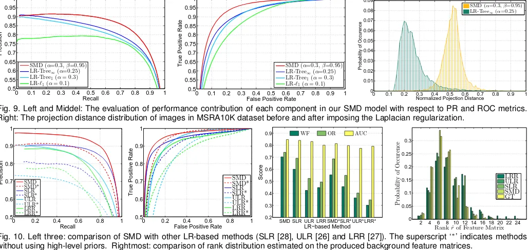
Fig. 9. Left and Middel: The evaluation of performance contribution of each component in our SMD model with respect to PR and ROC metrics. Right: The projection distance distribution of images in MSRA10K dataset before and after imposing the Laplacian regularization.
0 0.2 0.4 0.6 0.8 1 0.5
0.6 0.7 0.8 0.9 1
Recall
Precision SMD SMD* SLR SLR* ULR ULR* LRR LRR*
0 0.2 0.4 0.6 0.8 1 0.5
0.6 0.7 0.8 0.9 1
False Positive Rate
True Positive Rate
SMD SMD* SLR SLR* ULR ULR* LRR LRR*
SMD SLR ULR LRR SMD*SLR* ULR*LRR* 0.2
0.3 0.4 0.5 0.6 0.7 0.8 0.9
LR−based Method
Score
WF OR AUC
2 4 6 8 10 12 14 16 18 20 22 24 0
0.05 0.1 0.15 0.2 0.25 0.3
Rank ˆrof Feature Matrix
P
ro
b
a
b
ilit
y
o
f
O
cc
u
re
n
ce
[image:13.612.56.287.305.421.2]LRR ULR SLR SMD GT
Fig. 10. Left three: comparison of SMD with other LR-based methods (SLR [28], ULR [26] and LRR [27]). The superscript ‘∗’ indicates methods without using high-level priors. Rightmost: comparison of rank distribution estimated on the produced background feature matrices.
Image LR-`1 LR-Tree1 LR-Tree∞ SMD GT
Fig. 11. Saliency maps produced by variations of the SMD model.
in Appendix E and F.
5.3.3 Comparison with LR-based methods
We proceed to compare the proposed SMD method with other LR-based saliency detection methods on MSRA10K under two conditions: with and without high-level priors.
In the case of pure low-level saliency detection (i.e., without high-level priors), Fig. 10 shows that SMD consis-tently outperforms other LR-based methods in all metrics. In particular, the improvement of SMD over ULR [26] in-dicates that the integration of image structure information is superior to the learnt feature transformation in matrix decomposition.
When taking high-level priors into account, all the LR models are improved as validated in Fig. 10. SMD again achieves the best performance over all metrics. It indicates that both the structured regularization and high-level priors are beneficial for salient object detection.
Last, rank statistics of the background feature matrix
Lare collected for the above LR methods, as summarized
in Fig. 10 (rightmost). The results show that the matrices estimated by SMD achieve the lowest ranks among all the LR methods, and their rank distribution is similar to that calculated over the ground truth (GT). This implies that the structured-sparsity and Laplacian regularizations are complementary to the low-rank regularization in matrix
0.1 0.2 0.3 0.4 0.5 0.6 0.7 0.8 0.9 1 0.65
0.67 0.69 0.71
parameter α
WF score
0.2 0.4 0.6 0.8 1 1.2 1.4 1.6 1.8 2 0.69
0.695 0.7 0.705
parameter β
Fig. 12. The sensitivity analysis of parameterαandβ.
decomposition for estimating the intrinsic rank of image features.
5.3.4 Failure cases
Our method exploits the low-rank regularization to recover image background, therefore it may be difficult to suppress some small background regions with distinctive appear-ances, as shown in Fig. 13. The underlying reason is that the feature vectors of those regions are not in the low-dimensional subspace and may be incorrectly highlighted as foreground. Besides, for the salient objects with partial occlusion (see the third column in Fig. 13), SMD fails to con-sistently highlight the salient object because the constructed index-tree is not precise enough. Exploring more effective region grouping methods, such as [85], may alleviate this problem.