Proxy Simulation of In-Situ Bioremediation System
using Artificial Neural Network
Deepak Kumar
PhD Student
Civil Engineering Department, IIT Delhi-110016
Shashi Mathur
Professor
Civil Engineering Department, IIT Delhi-110016
ABSTRACT
In-situ bioremediation is one of the most economic techniques for groundwater remediation. BIOPLUME III is used to simulate the transport and biodegradation of contaminant. During optimal design of bioremediation system, the simulated BIOPLUME III data for the entire aquifer is usually called several times by optimization algorithm to optimize the system. This is a very time consuming process and thus there is a need of proxy simulator to be used in place of BIOPLUME III. Artificial neural network is used in the present study as proxy simulator. The results show that Levenberg-Marquardt back propagation technique can be used for training neural network and thus, ANN can be used as proxy simulators.
General Terms
Bioremediation, artificial neural network, groundwater, simulation
Keywords-
In-situ bioremediation, BIOPLUME III, optimization, neural network, back propagation, proxy simulator, groundwater1.
Introduction
Machine learning is a branch of artificial intelligence in which study of the system is done through learning from data. Machine learning studies automatic techniques for learning to make accurate predictions which are entirely based on past observations. Arthur Samuel [1] defined machine learning as a "Field of study that gives computers the ability to learn without being explicitly programmed". Artificial neural network (ANN), Support vector machine (SVM), Random forests are few examples of machine learning algorithms. ANN is widely used as machine learning tool in water resources problems. Aziz and Wong [2] were amongst the first to use an ANN approach for determining aquifer parameters from aquifer test data. A neural network was trained to recognize patterns of normalized drawdown as input data and the corresponding aquifer parameters as output data. Similarly, ANN was used for aquifer parameter estimation from pumping test data for a large diameter well by Balkhair [3]. Drawdown and well diameter data was used as input whereas transmissivity and storage coefficient were used as output data to train ANN. The results obtained by the proposed ANN method were
found to compare well with those obtained by the traditional curve fitting method. Likewise, ANN has been used remarkably by many researcher to train and test data in the resent past ([4], [5],[6], [7]).
Through such a simulator, the search problem becomes much simpler and quicker. A review of the literature shows that researchers have used the pattern recognition tools like ANN, SVM, GP etc. as proxy simulators in the past ([8]; [9]; [10]) in simulation models along with the optimization algorithms like simulated annealing, genetic algorithm, particle swarm optimization algorithm etc. Their results have shown that the computational time can be significantly reduced by using proxy simulators. Also, combination effectively reduces the computational burden of the overall problem. In the present study, ANN is modelled as a proxy simulator in place of BIOPLUME III.
2.
Study Area
A hypothetical site which is contaminated with BTEX (Benzene, Toluene, Ethylbenzene and Xylene) is used in the present study for simulating biodegradation using BIOPLUME III. BTEX is a compound released from petroleum site and by leaching, it pollute the groundwater. The hydrological properties of the contaminated site are shown in Table 1. From Table 1, it may be noted that the initial maximum concentration of BTEX is 40 ppm. Three years of remediation period is selected and at the end of 3 years, allowable concentration of 5 ppm is expected from the entire aquifer.
Table1. Hydrological property of the hypothetical site
Aquifer property Value
Hydraulic Conductivity 6 x 10⁻⁶m/s Hydraulic gradient 0.005
Transverse dispersivity 1m
Longitudinal dispersivity 8m
Effective porosity 0.3
Anisotropic factor 1
Total remediation period 3
Initial BTEX concentration 40 ppm
To remediate this site, in-situ bioremediation is adopted. For in-situ bioremediation, set of injection and extraction wells are needed as shown in Fig.1. Injection wells are installed in the up gradiant site of groundwater flow where as extraction wells are installed in the down gradient side of groundwater and contaminant flow. Through injection well excess of oxygen and other nutrient is provided to the microbes which are present in the aquifer. These microbes consume BTEX in presence of oxygen. In this way, contaminant concentration decreases slowly and gradually. Extraction wells are installed to check the movement of contaminant water towards the monitoring wells. Extraction wells also accelerate the rate of biodegradation of contaminant. In
and one extraction well (e1) is used for in-situ bioremediation.
Fig.1. BTEX contaminated site
3.
Governing Equations
In the present study, BIOPLUME III uses equation 1 and equation 2 for modeling bioremediation in-situ bioremediation in which Instantaneous reaction kinetics has been used. Use of instantaneous model is proposed by Borden and Bedient [11]. The instantaneous reaction model has the advantage of not requiring kinetic data.
(1)
(2)
Where, C = concentration of hydrocarbon; O = concentration of oxygen; C’ =concentration of hydrocarbon in source or sink; O’ = concentration of oxygen in source or sink; η = effective porosity; b = saturated thickness; W = volume flux per unit area; Vi =seepage velocity in the direction of xi;Rh =retardation factor for hydrocarbon; Di j=coefficient of hydrodynamic dispersion; xi, xj= cartesian coordinates; t = time.
4.
Methodology
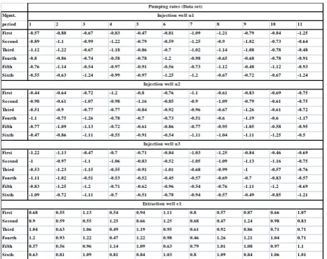
dioxide [12]. To enhance bioremediation process in BIPLUME model, set of injection and extraction wells are used. Pumping rates for injection and extraction wells are randomly generated between 0.5 ls-1 and 1.25 ls-1. To manage the pumping rate optimally, three years of remediation period is divided into six management period. Each management period is of six months. During a management period, the pumping rate is fixed and the pumping rate only change with change in management period. 500 data sets for pumping rate are generated between 0.5 ls-1 and 1.25 ls-1 both for injection and extraction wells during six management period. A sample of data set is shown in Table 2. In Table 2, only 11 data sets are shown. Likewise, 500 data sets has been randomly prepared and for each data set of pumping rates, maximum BTEX concentration is determined after three years of remediation period with the help of BIOPLUME III.
Table 2 Sample data set of pumping rates for three injection and one extraction well
To simulate ANN as proxy simulator, pumping rate is considered as input data and maximum allowable concentration obtained from BIOPLUME is considered as output data. Fig. 2 shows the flow chart for simulating ANN as proxy simulator. 500 data set for pumping rate data acts as input data for training ANN. Also, the pumping rate from each data set is used to simulate BIOPLUME III for getting maximum contaminant concentration after three years of remediation. The obtained maximum contaminant concentration acts as output data or target data for training ANN.
Fig.2 ANN as proxy simulator
The configuration of a neural network is determined by the number of input variables, hidden neurons, and outputs as well as the number of layers of hidden neurons. In the present study, artificial neural network is developed using Levenberg-Marquardt back propagation algorithm. Back-propagation which is a supervised training algorithm is by far one of the most commonly used methods for training neural network [13]. Neural network toolbox of MATLAB is used to configure the algorithm. The network used in the present study is shown in Fig.3. As shown in Fig.3, two layers of hidden neurons are used.Tan-sigmoid transfer function is used in the hidden layer 1 and linear transfer function in the outer layer 2.
Fig.3 Neural network configuration
Pumping rates is used as input variable whereas maximum BTEX concentration is used as output variable for training neural network. 20 neurons for first hidden layer are selected for computational work. 0.5 is selected as learning rate.
5.
Results and discussion
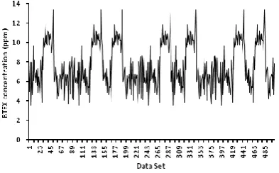
The main aim of this study is to develop a proxy simulator in place of BIOPLUME III. With the help of BIOPLUME III, maximum BTEX concentration in the aquifer after three years of remediation period is obtained for 500 data sets of time varying pumping rates during six management period which is shown in Fig.4.
Mgmt.
pe riod 1 2 3 4 5 6 7 8 9 10 11
First -0.57 -0.88 -0.67 -0.83 -0.47 -0.81 -1.09 -1.21 -0.79 -0.84 -1.25 Se cond -0.89 -1.1 -0.99 -1.22 -0.79 -0.59 -1.25 -0.9 -1.02 -0.73 -0.64 Third -1.12 -1.22 -0.67 -1.18 -0.86 -0.7 -1.02 -1.14 -1.08 -0.78 -0.48 Fourth -0.8 -0.86 -0.74 -0.58 -0.78 -1.2 -0.98 -0.65 -0.68 -0.78 -0.91 Fifth -0.76 -1.14 -0.54 -0.97 -0.91 -0.56 -0.73 -1.12 -0.48 -1.12 -0.93 Sixth -0.55 -0.63 -1.24 -0.99 -0.97 -1.25 -1.2 -0.67 -0.72 -0.67 -1.24
First -0.44 -0.64 -0.72 -1.2 -0.8 -0.76 -1.1 -0.61 -0.83 -0.69 -0.75 Se cond -0.98 -0.61 -1.07 -0.98 -1.16 -0.85 -0.9 -1.09 -0.79 -0.61 -0.75 Third -0.51 -0.9 -0.77 -0.77 -0.84 -0.92 -0.96 -0.67 -1.26 -0.61 -0.72 Fourth -1.1 -0.75 -1.26 -0.78 -0.7 -0.73 -0.51 -0.6 -1.19 -0.6 -1.17 Fifth -0.77 -1.09 -1.13 -0.72 -0.61 -0.86 -0.77 -0.95 -1.05 -0.58 -0.95 Sixth -0.47 -0.86 -1.11 -0.55 -0.91 -0.54 -1.11 -1.04 -1.11 -1.25 -0.5
First -1.22 -1.13 -0.47 -0.7 -0.71 -0.84 -1.03 -1.25 -0.84 -0.46 -0.69 Se cond -1 -0.97 -1.1 -1.06 -0.83 -0.52 -1.05 -1.09 -1.13 -1.16 -0.75 Third -0.53 -1.23 -1.15 -0.55 -0.91 -1.01 -0.68 -0.99 -1 -0.57 -0.76 Fourth -1.11 -1.02 -0.51 -0.53 -0.52 -0.45 -0.57 -0.69 -0.7 -0.83 -0.57 Fifth -0.83 -1.25 -1.2 -0.71 -0.62 -0.96 -0.54 -0.76 -1.11 -1.2 -0.69 Sixth -1.09 -0.72 -1.11 -0.7 -0.51 -0.78 -0.94 -0.57 -0.49 -0.85 -1.21
First 0.68 0.55 1.13 0.54 0.94 1.11 0.8 0.57 0.87 0.66 1.07 Se cond 0.9 0.59 0.55 1.25 0.66 1.25 0.68 0.47 1.24 0.98 0.83 Third 1.04 0.63 1.06 0.49 1.19 0.95 0.61 0.92 0.86 0.71 0.71 Fourth 1.2 0.93 1.22 0.47 1.22 0.98 0.46 1.26 1.21 1.04 0.71 Fifth 0.57 0.56 0.96 1.14 1.09 0.63 0.79 1.01 1.08 0.97 1.1 Sixth 0.63 0.81 1.09 0.81 0.84 1.03 0.8 1.09 0.84 1.06 1.01
Pumping rate s (Data se t) Inje ction we ll u1
Inje ction we ll u2
Inje ction we ll u3
[image:3.595.325.534.74.186.2] [image:3.595.41.274.316.500.2] [image:3.595.323.536.396.453.2]Fig.4 Maximum BTEX concentration for 500 pumping dataset using BIOPLUME III
Considering time varying pumping rates as input data and maximum BTEX concentration in the aquifer as the output data, the developed neural network has been run for 20 times to get most accurate coefficient of regression between the input and output data. The coefficient of regression for the training data set, validating data set and testing data set is shown in Fig. 5a, Fig. 5b and Fig. 5c respectively. In case of raining and testing data set, the coefficient of regression is nearly close to 1 which indicates that the data set is properly trained. The overall coefficient of regression is 0.976 which shows a strong correlation between input and output data set.
Fig.5 Regression analysis for training, validating and testing ANN
The performance of configured artificial neural network is shown in Fig. 6. Mean square error of training, testing and validating data sets is plotted against the total number of epochs. From this figure, it is clear that as the number of epochs is increasing, the mean square error is decreasing. The best validation performance is 0.8594 which is obtained at epoch 6.
Fig. 6 Performance of configured neural network
The output obtained from the trained artificial neural network for 500 data sets of pumping rates is shown in Fig.7. The output data obtained from BIOPLUME III and trained ANN is compared in Fig.8. The coefficient of correlation between these two outputs is 0.9978 which is shown in Fig.8. The strong correlation between
BIOPLUME III and trained ANN shows that trained neural network can be used as proxy simulators.
Fig.7 Maximum BTEX concentration for 500 pumping dataset using trained ANN
Fig.8 Comparison between BIOPLME III and Trained ANN
6.
Conclusion
During solving complex optimization problems, proxy simulators are often used in place of real simulators which significantly reduce the computation time to reach the global optima. In this study, artificial neural
y = 1.0004x + 0.0028 R² = 0.9978
-1 4 9 14
-1 4 9 14
Tr
ai
n
e
d
A
N
N
[image:4.595.333.522.75.224.2] [image:4.595.68.265.77.199.2] [image:4.595.313.502.331.459.2] [image:4.595.69.268.400.562.2] [image:4.595.318.537.524.652.2]of BIOPLUME III. The results show that Levenberg-Marquardt back propagation technique can be used as developing proxy simulator with high performance.
7.
Acknowledgements
Author is thankful to the civil engineering department of Indian institute of technology, Delhi for providing the necessary simulation laboratory facility needed for the study.
8.
References
[1] Samuel, A. 1959. Some studies in machine learning using the game of checkers. IBM Journal of Research and Development, 3(3):210–229.
[2] Aziz, A. and Wong, K. (1992). “Neural-Network Approach to the Determination of Aquifer Parameters.” Ground Water GRWAAP,, 30(2).
[3] Balkhair, K. (2002). “Aquifer parameters determination for large diameter wells using neural network approach.” Journal of Hydrology, 265(1-4), 118–128.
[4] Chang, L. and Chang, F. 2001. Intelligent control for modelling of real-time reservoir operation.
Hydrological Processes, 15(9), 1621–1634.
[5] Coppola Jr, E., Rana, A., Poulton, M., Szidarovszky, F., and Uhl, V. 2005. A neural network model for predicting aquifer water level elevations. Ground Water, 43(2), 231–241.
[6] Prasad, R. and Mathur, S. 2006. “In-Situ Bioremediation of Contaminated Groundwater Using Artificial Neural Network.” ASCE.
[7] Muttil, N. and Chau, K. 2007. “Machine-learning paradigms for selecting ecologically significant
input variables.” Engineering Applications of Artificial Intelligence, 20(6), 735–744.
[8] Morshed, J. and Kaluarachchi, J. J. 1998a. Application of artificial neural network and genetic algorithm in flow and transport simulations. Advances in Water Resources, 22(2), 145–158.
[9] Aly, A. H. and Peralta, R. C. 1999. “Optimal design of aquifer cleanup systems under uncertainty using a neural network and a genetic algorithm.” Water Resour. Res., 35(8), 2523–2532.
[10]Johnson, V. M. and Rogers, L. L. 2000. Accuracy of neural network approximations in simulation-optimization. Journal of Water Resources Planning and Management, 126(2), 48–56.
[11]Borden, R.C., Bedient, P.B. 1986.Transport of dissolved hydrocarbons influenced by oxygen-limited bioremediation. 1. Theoretical development. Water Resources Research, Vol.22, No.13, Pages 1973-1990
[12]Rifai, H. S., Newell, C. J., Gonzales, J. R., Dendrou, S., Kennedy, L., and Wilson, J. T. 1997. BIOPLUME III natural attenuation decision support system, version 1.0, user’s manual. Air Force Center for Environmental Excellence (AFCEE), San Antonio.