Performance Evaluation of Stereo Matching Algorithms in the Lack of Visual Features

Performance Evaluation of Stereo Matching Algorithms

in the Lack of Visual Features

Mohammed Ouali

LITIO Lab, B.P.1524 Elmenaouer, Oran, 31000, Algeria

College of C.I.T., Dept. of Computer Engineering, Taif University, K.S.A.

ABSTRACT

In this paper, we evaluate three different subcategories of image matching algorithms. We consider hierarchical matching, wavelet-based localized correlation and multiresolution subregioning. The importance of this evaluation stems from the fact that these algorithms are all somehow based on a multiresolution scheme, but exhibit different performances when dealing with featureless image pairs, noisy image pairs, or when tuned to different parameters, e.g. the number of resolution levels and the size of the correlation size. We also consider the use of different correlation functions. A data set has been built using random dots stereograms, with a full range of disparities and a controlled amount of noise. The algorithms performances are benchmarked in terms of accuracy and global coherence of the disparity maps.

General Terms

Machine vision, stereo matching, performance evaluation.

Keywords

Stereo matching, performance evaluation, wavelets-based design, window-based matching algorithm, hierarchical algorithms.

1.

INTRODUCTION

Human vision provides information regarding surrounding objects and allows taking actions based on the environment. Human vision not only provides information on objects features, like color and texture, but also to perceive shape of objects, their location with respect to each other and to the observer, their motion, and so forth. One of the toughest tasks in machine vision is the 3D reconstruction of a scene from one or several images. We are particularly interested in the case of stereo where two or three cameras observe a scene.

Stereo vision is a fundamental precursor to 3D reconstruction, robot navigation, and obstacle avoidance to name a few [2,9]. The technique is based on the use of two cameras on a stereo rig that observe a scene. The scene projections on the cameras are not exactly identical since the cameras do not have the same spatial location. This results in horizontal and vertical shifts, called disparity that encode objects' depth: a farther object will have a small shift while a closer object will produce a large shift in the stereo images. The key aspect of 3D vision is the stereo image matching to produce disparity maps (maps that contain spatial shifts for each pixel). However, disparity maps do not allow the knowledge of the 3D structure of the observed scene [10]. For this, one needs to know the stereo rig parameters, namely, image size, pixel size, focal length, relative orientation of stereo cameras and the baseline distance between the cameras.

By matching the stereo images, we can compute disparities (horizontal and vertical image shifts of corresponding visual features). Using the disparity maps along with stereo rig parameters, it is straightforward to calculate the Euclidean structure of the scene. The major problem here is the matching of the stereo images to build disparity maps and the recovery of accurate stereo rig parameters, namely extrinsic and intrinsic camera parameters, that could be determined through a calibration procedure.

Image matching has been an active research topic in the last three decades and several authors have proposed approaches and algorithms. Most of these approaches are based on matching visual features, represented as contours delimiting objects, regions describing objects or areas, or points representing image pixels and encoding the luminance of the objects in the scene. The proposed algorithms in the literature use optimization as a resolution method, the gray level correlation, correlation of discrete features such as edges and regions, wavelet decomposition, hierarchical Burt’s pyramid (based on Gaussian or square window) to name a few [13]. Some other works suggested that the inference of 3D structure and disparity is independent of the existence of such visual features, and the disparity is only related to structural relationship between stereo images. Among these methods, we cite cepstral, phase-based, and phase difference-based approaches [4—6]. While these approaches are able to produce coherent disparity maps with sub pixel accuracy, they do not use visual features as a matching feature, either explicit or implicit, except maybe for the phase correlation approach, where phase might be considered as an implicit visual feature. Moreover, these approaches have been used to successfully match random dot stereograms (RDS). Most importantly, certain algorithms are noise sensitive by design, while others need to be evaluated in presence of controlled noise.

In this work, we want to benchmark the performances of certain visual features-based algorithms [3,7,11]. We examine how visual features-based algorithms deal with RDS, since RDS exhibit a repetition of random patterns that could mislead the matching algorithm. Finally, we want to assess the impact of noise on these algorithms as well as algorithms' parameters such as the correlation window size and the correlation function. We selected three algorithms pertaining to different approaches: hierarchical matching [1], multiresolution sub-regioning and dynamic programming [8], and a wavelet-based localized correlation function matching [12].

2.

MATCHING ALGORITHMS

Hierarchical matching (HM) is based on the construction, for each image, of a pyramid of images: the top of the pyramid corresponds to the lower resolution, while the base of the pyramid is higher resolution image corresponding to the original image. Without loss of generality, one can use a Gaussian window or any other window to form the pyramid. Starting from the top of the pyramid, lower resolution images are matched. The disparity map obtained is used in the next resolution to verify and to predict new matching. This process is repeated until the full resolution images at the base of the pyramid are matched, hence, obtaining the final disparity map.

The multiresolution subregioning-based matching (MSM) consists of trying a range of disparities and using several correlation windows. For each disparity, a correlation window of a given size is used to compute a correlation function. A correlation cube is built for each window size. The width and height of the cube are identical to those of the images to be matched. The depth axis corresponds to the disparity. Each vertical slice of the cube corresponds to correlation scores obtained at a given disparity. A horizontal slice of the cube shows, for an image line, the correlation scores at different disparities. The final disparity map is obtained by finding for each image line the smoothest path having the maximum correlation scores at each image location.

The wavelet-based localized correlation function matching algorithm (WLCM) decomposes both stereo images using the Laplacian of Gaussian wavelet (LoG). A correlation kernel is also defined according to the LoG wavelet. The correlation kernel takes the image information at all scales to compute the correlation score. A simpler description of this algorithm is the construction of a vector for each pixel; the vector contains the multiscale information computed by the wavelet decomposition. The scalar product scores are used as a confidence score to validate the matching of two given pixels.

3.

EVALUATION PROTOCOL

3.1

Noiseless Random Dots Stereograms

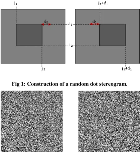
RDS are generated as random dots to describe surfaces. Surfaces may be shifted to create disparities. Complex depth planes can be constructed while not having any visual features. The matching of such RDS is possible by human subjects: the observer squints to superimpose both images and then focuses at several depths to adjust the correct depth at which the hidden structure in the RDS comes up. In the figure below, we show how a stereogram is built: the dark square represents a surface on a background; the square is positioned at different locations in both images (left and right).

One important byproduct of using random dots stereograms is the exact knowledge of the disparity map, also called reference disparity map. The reference disparity map is used to determine the accuracy and the correctness of the computed disparity maps by the algorithms under consideration.

The RDS used in this study are 256x256 pixels. The structure embedded within the streogram is 64x64 pixels. Each RDS is built by shifting the structure (every pixel making the structure) by a constant shift (the disparity). We produced 17 stereograms representing disparities from 4 to 20 pixels.

Fig 1: Construction of a random dot stereogram.

Fig 2: Left and right hand side images of a stereogram.

3.2

Noisy Random Dots Stereograms

Similarly, for each disparity, we produced noisy stereograms. The noisy stereogram is produced by adding a white Gaussian noise to one of the images of the stereo pair. The figure below shows a stereogram with the right image corrupted with noise—note the photometrical imbalance between the images.

Fig 3: RDS with the right image corrupted with white Gaussian noise.

3.3

Evaluation Criteria

In order to evaluate the disparity estimation algorithms, we consider the absolute error between the computed disparity map and the reference disparity map

| ( ) ( )|

where ( ) is the computed map and ( ) is the

reference disparity map. We also consider the percentage of correct matches ( ), the percentage of acceptable matches ( ), and the percentage of erroneous matches ( ). Moreover, we consider the average absolute error and the root mean square error for the whole disparity map, defined by

_√ ∑ ∑| ( ) ( )|

where is the disparity map size. Finally, the average relative error, that is given by

∑ ∑| (

₎

( )|

( )

4.

EXPERIMENTAL RESULTS

The experimentations consist of evaluating the above mentioned criteria, and particularly

1. the average absolute error; 2. the average relative error;

3. the percentage of correct matches (error less than one pixel.

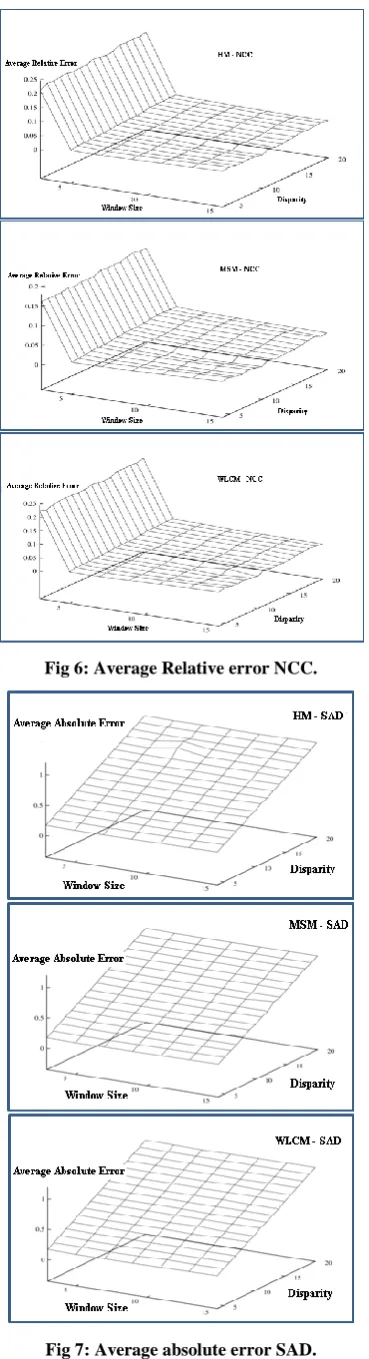
We consider both noisy and noiseless RDS in the experimentations. We also consider RDS with disparities varying from four to 16 pixels. The correlation window size have been varied from 3x3 to 15x15. The correlation functions that have been considered are the sum of absolute differences (SAD), the sum of squared differences (SSD), and the normalized cross-correlation (NCC).

Figures 4, 5, and 6 show the average relative error when SAD, SSD, and NCC are used. For plot presented in this part, the following concepts are used. It clearly visible that the error is significant when a small window is used in presence of large disparities, which confirms the common knowledge in the field. Otherwise, there is a minimum in the error surface when the window size corresponds to the preponderant disparity in the stereo pair. Finally, the multiresolution subregioning matching algorithm (MSM) produces a smoother error surface indicating a stability with respect to the fluctuations of the window size and the disparity.

Figures 7 and 8 show the average absolute error for SAD and NCC correlation functions. The absolute error varies linearly with respect to the disparity. However, it does not vary with respect to the window size. Almost no differences are reported between SAD and NCC absolute errors, although NCC provides better results than SSD in terms of relative error; similarly, SSD provides better results than SAD in terms of relative errors.

Figure 9 shows the percentage of correct matches for different algorithms using different correlation functions. Generally speaking, the trend is the same: the percentage of correct matches degrades when small window sizes are used in presence of large disparities. Otherwise, the percentage of correct matches varies little or not at all. Window sizes around 13x13 proved successful in retrieving the correct disparity and the maximum percentage of correct matches is nearly 89%. The results are shown for stereo pairs with 20% of the image pixels corrupted with noise.

Finally, it is noted that MSM algorithm gives better results when used with the normalized cross-correlation, whereas, the HM and WLCM algorithms produce their best estimates with and SSD.

Fig 4: Average relative error SAD.

Fig 6: Average Relative error NCC.

Fig 7: Average absolute error SAD.

Fig 8: Average absolute error NCC.

5.

CONCLUSION

In this paper, we evaluated the performance of some stereo matching algorithms. An experimental protocol for producing and comparing their performances has been put in place. The evaluation protocol allowed us to characterize the behavior of each algorithm: accuracy, robustness to noise, robustness to algorithm parameters. We used a data set for noiseless and noisy RDS, with disparities varying from four up to 16 pixels. This study shed more light on the understanding of some of most important matching techniques.

Although, in this work, we considered stereograms contaminated with noise, extension of this work might consider other degradations such as scale change, difference in contrast, and camera imbalance effects. This will help better benchmarking the performances of stereo matching algorithms in the lack of visual features.

6.

ACKNOWLEDGMENTS

This work was partly financially supported by a LITIO Lab and University of Taif research grant (2061-433-1). The author would like to thank Ms. K. Hadj Djelloul for her help in creating the data sets used in this study.

7.

REFERENCES

[1] Roberto Brunelli. Template Matching Techniques in Computer Vision: Theory and Practice, John Wiley & Sons, Ltd., 2009.

[2] Jyothi Digge and Yashraj Digge, Stereo vision for Robotics. IJCA Proceedings on International Conference and workshop on Emerging Trends in Technology (ICWET 2012), pp. 33-39, 2012.

[3] Hirschmuller, H., and Scharstein, D., Evaluation of stereo matching costs on images with radiometric differences. IEEE Transactions on Pattern Analysis and Machine Intelligence, 31(9):1582-1599, 2009.

[4] Ouali, M. and Laurgeau, C., A cooperative multiscale phase-based disparity algorithm. IEEE ICIP (3) 1999: 145-149.

[5] Ouali, M. and Laurgeau, C., Dense Disparity Estimation Using Gabor Filters and Image Derivatives. IEEE 3DIM 1999: 483-489.

[6] Ouali, M., Lange, H., and Laurgeau, C., Energy minimization approach to dense stereo vision. IEEE ICIP (2) 1996:841-845.

[7] Rachna, H S Singh and A K Verma. Article: Segment Controlled Window Shape to Compute Disparity Map from Stereo Images. IJCA Special Issue on Electronics, Information and Communication Engineering ICEICE(4):38-41, December 2011.

[8] Sun, C., Fast stereo matching using rectangular subregioning and 3D maximum surface techniques. International Journal of Computer Vision, Vol. 47, pp. 99-117, 2002.

[9] Szeliski, R., Computer Vision: algorithms and applications. Springer, 2010.

[10]R. Szeliski and D. Scharstein. Sampling the disparity space image. IEEE Transactions on Pattern Analysis and Machine Intelligence, 26(3):419-425, March 2004.

[11]R. Szeliski, R. Zabih, D. Scharstein, O. Veksler, V. Kolmogorov, A. Agarwala, M. Tappen, and C. Rother, A comparative study of energy minimization methods for Markov random fields with smoothness-based priors. IEEE Transactions on Pattern Analysis and Machine Intelligence, 30(6):1068-1080, 2008.

[12]Perrin, J., Torresani, B., and Fuchs, P., A localized correlation function for stereoscopic image matching. Traitement du Signal, Vol. 16, Issue 1, 1999.