Evaluation of Direct and Derived Mobility Metrics of
Mobility Models and Their Impact on Reactive Routing
Protocols
Santosh Kmuar
S.C.Sharma
Indian Institute of Technology, Indian Institute of Technology,
Roorkee (India) Roorkee (India)
ABSTRACT
Mobile Adhoc Network (MANET) routing protocols performance are perceptive to mobility and scalability of network, therefore, the objectives of paper is to describe mobility models based on mobility matrices class and impact of these metrics on routing performance metrics in MANET. An effort for analyzing derived mobility metrics with direct mobility metrics are considered across mobility models i.e. Random waypoint, Reference Point Group, Manhattan, Freeway in this article. This article focuses impact analysis of mobility models on two prominent reactive routing protocols i.e. ad-hoc on demand distance vector (AODV) and dynamic source routing (DSR) with fixed network size, varying node speed and identical traffic load and also extends an intuitive study to analysis the interplay between mobility patterns and protocols building blocks.
Keywords
Mobility models, mobility metrics, connectivity graph metrics, routing protocol-AODV, DSR and routing metrics.
1. INTRODUCTION
Mobile Adhoc Network (MANET) is a collection of mobile nodes forming a temporary network, without the aid of pre-establishment network infrastructure. Although, commercial wireless technologies are generally based on towers and high-power base stations [1, 2]. They are fixed in location and relationship to their client devices. Many researchers have shown their interest in the field of MANET and all sorts of protocols aiming at different issues. The performance of these protocols need to be carefully evaluated before they are ready for the commercial market, so for network simulation plays vital role as well as a key method to comprehend the overall performance of the MANET. The performance of these protocols could be evaluated with the imperative mobility model that precisely represents mobile nodes (MNs) to provide realistic performance measurement. In mobility modeling research, there are two direction of research which could be performed. First direction is towards designing of new model which predicts new era of real world scenario. Second direction is to analyze mobility models on account of mobility metrics and influences of mobility models on routing protocols. There are many mobility models have been proposed in the literature (3, 4, 5, 6, 7, 8, 9). Brief descriptions of some mobility models are taken i.e. Random waypoint, Reference point group, Manhattan and freeway.
This paper basically evaluates mobility metrics and connectivity graph metrics for providing a frame work which is helpful for understanding and evaluating the impact on routing protocols performance like AODV and DSR [10, 12,
13] based on routing protocols metrics as well as an intuitive study to analyze the interplay between mobility patterns and protocols building blocks.
2. BRIEF DESCRIPTION OF MOBILITY
MODELS
Brief descriptions of some mobility models are taken i.e. Random waypoint, Reference point group, Manhattan and Freeway.
Random Waypoint Model (RWPM): It includes pause times between changes in direction and speed. A mobile node (MN) stays in one location for certain period of pause time [13].
Reference Point Group Mobility Model (RPGM): A group mobility model where group movements are based upon the path travelled by a logical centre. Group mobility can be used in military battlefield communications where the commander and soldiers form a logical group and many more [14].
Manhattan Grid Model (MGM): In this model nodes move only on predefined paths. The arguments -u and -v set the number of blocks between the paths [6, 17]. Freeway: This model emulates the motion behavior of
mobile nodes on a freeway map and each freeway has lanes in both directions [6]. It can be used in exchanging traffic status or tracking a vehicle on a freeway.
3. MOBILITY METRICS
Mobility matrices were first introduced by P. Johansson et al. [16]. To differentiate various mobility patterns and these mobility pattern Qunwei Zheng et al. [15] classify mobility metrics in two categories: direct and derived metrics. First evaluates the phenomena of clear physical correspondence (such as speed or acceleration) like the temporal dependence, spatial dependence and geographic restrictions. In addition to these metrics, the relative speed metric that differentiates mobility patterns based on relative motion. Second uses mathematical modeling to measure the change to some logical structure (e.g. connectivity graph). The other metrics which is included in this paper is routing performance metrics. These metrics are used to analyze the impact of mobility on routing protocols performance metrics in MANET.
The metrics classification is visualized broadly into two categories as:
Mobility metrics
Protocol performance metrics
3.1 Direct Mobility Metrics
Random Based: Characteristics of this metrics have no dependencies and restriction. This metrics has statistical model, in this node can move to any destination and their velocities and directions are chosen randomly. These models are basically idealistic rather than realistic, because in a real world, nodes move randomly without any destination.
[image:2.595.316.541.571.719.2]Relative Speed (RS): It is standard definition drawn from physics which is based on relative speed [6, 17] of all pairs of nodes in networks over time t i.e. the speed of first node i, relative to the second node j.
( , , ) | ( ) ( ) | (1)
RS i j t V ti V tj
Average Relative Speed:Average relative speed RS (i, j) of hosts i, j at time t will be-
( , , )
1 1 1
(2)
N N T
RS i j t
i j t
RS
P
where P is the number of tuples (i, j, t) such that RS(i, j, t) ≠ 0.
Degree of Temporal Dependence: The temporal
dependencies imply how an individual node changes its velocity with respect to time or a node actual movement influenced with its past movement. For each node, it is defined as a product of relative direction and relative speed (relative to its past itself) i.e.
( , , ') ( ( ), ( ')) ( ( ), ( ')) (3)
Dtempi t t RD v t v ti i SR v t v ti i
The value of Dtemp (i, t, t’) is high when node moves in the same direction and almost at similar speed and decreases if relative direction or the speed ratio decreases over a certain time interval. 0 ) t' t, ( i, temp D c | t' t |
where c > 0 is a constant
Average Degree of Temporal Dependence: The average degree of temporal dependence Dtemp (i, t, t’) is the value of averaged over nodes and time instants i.e.
(4)
N T T D (i, j,t')
temp i=1 t=1 t'=1 Dtemp=
P
where P is the number of tuples (i, t, t’) such that Dtemporal (i, t, t’) ≠ 0. It has two conditions that is obvious, first, if the present velocity of a node is fully independent of its velocity at previous time period, then the mobility pattern is expected to have a smaller value for Dtemporal . Second, if the current velocity is strongly dependent on the velocity at some previous time step, then the mobility pattern is expected to have a higher value for Dtemporal.
Degree of Spatial Dependence: The degree of spatial dependence is a measure of a node‟s correlation with others nodes in the networks. The degree of spatial dependence between nodes i, j, at time t (Dspatial(i , j, t)) by equation 5.
(5)
D (i, j,t)= RD(v (t),v (t))* SR(v (t),v (t))i j i j spatial
The value of Dspatial ( i , j, t) will increases when nodes i and j move in same direction with almost similar speed and decreases when nodes i and j move in relative direction or dissimilar speed over certain time interval. The spatially dependent on a far away node will be zero and satisfy following conditions i.e.
0 t) j, ( i, spatial D R c ( t) j i,
D
where c > 0 is a constant.
Average Degree of Spatial Dependence: The average degree of spatial dependence is an average of degree of spatial dependence of all nodes pairs in the network [5] i.e.
(6)
T N N D (i, j,t) t=1 i=1 j=i+1 spatial
D =
spatial P
where P is the number of tuples (i, j, t) such that Dspatial(i, j, t) ≠ 0.
3.1.1 Evaluation of Direct Metrics for Mobility
Pattern Differentiation
Direct metrics evaluation leads for the differentiation of mobility patterns. For this, differentiation a mobility pattern scenario is required which captures the characteristics of relative speed, temporal dependence and spatial dependence. A user manual for IMPORTANT Mobility Tool Generators in NS-2.34 simulator is used [17]. This mobility tool is owned by ProTest Lab, Univ. of Southern California., where it serves as a tool for the investigation of mobile adhoc network characteristics. This tool is useful for creating and analyzing mobility metrics.
3.1.2 Simulation Environment Setup
A mobility scenario generator produced different mobility patterns for mobility model i.e. Reference Point Group Mobility Model (RPGM), Random Waypoint Model (RWPM), Freeway mobility model (FMM) and Manhattan Mobility model (MMM). The scenario generator creates scenario file with respect to parameters. The common scenario parameters for these models are- transmission range is 250 m, simulation area 1000m x 1000m, number of nodes is 40, Max speed (Vmax) are 1,5,10, 20, 30, 40,50, 60 m/sec and simulation duration is 900sec. some other parameter which are specifically taken, max pause (p) is 20s for RWPM, speed deviation ratio (SDR) & angle deviation ratio (ADR) are 0.1 for RPGM (SG&MG) and for Manhattan mobility model (MMM) minimum allowed velocity & acceleration speed are 0.5. The simulation setup is created over Fedora 11 (Linux- Platform) environment for direct metrics and derived metrics analysis, shown in Fig. 7.
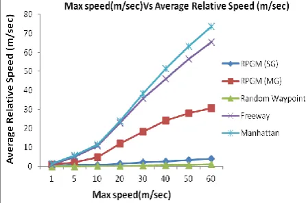
Average relative speed: It has been observed from the simulation that the average relative speed of Random Waypoint Model (RWPM) almost linear as the Vmax increases and has lowest value.
Fig. 2 Max speed (m/sec) Vs Average Degree of Temporal Dependence
RPGM (SG) has lowest value for relative speed as compared to Freeway, Manhattan mobility models, as its nature of group movement pattern while RPGM (MG) of 10 nodes has more value than RPGM (SG) because it has behavior of relative group movement of each group and has almost same value at end of simulation as shown in fig. 1. Average Relative speeds of Manhattan and Freeway mobility model have higher value as the Vmax increases.
The results analysis of average degree of temporal dependence causes uncertainty for differentiation of different mobility pattern in study as shown in fig. 2. The usefulness of this metrics is still in research.
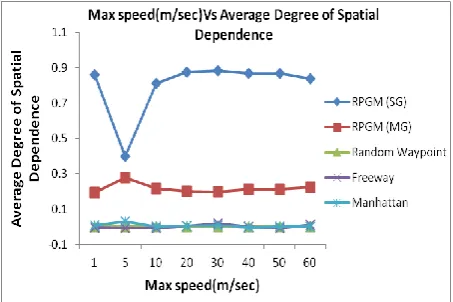
The average degree of spatial dependence is high in RPGM (SG) of 40 nodes, RPGM (4- groups) of 10 nodes respectively, it is because the group leader monitors the movement of mobile node. Therefore, RPGM (SG & MG) has high spatial dependence. In the case of Random Waypoint, Freeway and Manhattan have almost 0 as shown in fig. 3.
Fig. 3 Max speed (m/sec) Vs Average Degree of Spatial Dependence
Finally, this section concludes with analysis result and validates direct mobility metrics for mobility pattern. This section classifies the mobility model by evaluation of mobility metrics (direct metrics) from fig. 1-3, and differentiates them by consideration of mobility patterns in an evocative & systematic fashion. The results shown in fig. 1 differentiate performance of those models which do not belongs the class of random based metrics (i.e. RPGM, freeway, Manhattan), are affected because these are having some dependencies as well as restrictions. Average relative speed of RWPM has
small value than Manhattan, Freeway and RPGM (SG &MG) mobility model respectively as the Vmax increases. The temporal dependency causes uncertainty for differentiation of different mobility patterns and finally RPGM (SG & MG) has high spatial dependence.
3.2
Effect evaluation of Mobility Model on
Connectivity
Graph
Metrics
(Derived
metrics)
This metrics is derived from graph theoretic models as well as other mathematical models. Mobility model impact the connectivity graph which in turn influence the protocol performance. Therefore, it is necessary to study metrics that capture the properties of connectivity graph.
Connectivity Graph: The connectivity graph is the graph G= (V, E) where |V|=N, a link (i, j) ϵ E iff Di, j (t)≤ R. Let X(i, j, t) be an indicator random variable which has a value 1 iff there is a link between nodes i and j at time t.
t) j, X( i, T
1 t max j)
X( i, be an indicator random variable which is 1 if a link existed between nodes i and j at any time during the simulation, 0 otherwise. The graph connectivity metrics includes number of link changes, link duration and path availability. The connectivity graph metrics and their brief descriptions are as [5, 6, 12, 18, 19].
Number of Link Change
Number of link changes (LC) for a pair of nodes i and j is the number of times the link between them transitions from “down” to “up” and defined as-
(7) T
LC(i, j)= C(i, j,t) t=1
where C(i, j, t) is indicator random variable such that C(i, j, t) = 1 iff X(i, j, t − 1) = 0 and X(i, j, t) = 1 i.e. if the link between nodes i and j is down at time t − 1, but comes up at time t.
Average Number of Link Changes
Average Number of Link Changesis the value of LC (i, j) averaged over node pairs satisfying certain condition i.e.
(8)
N N
LC(i, j) i=1 j=i+1 LC
P
where P is the number of pairs i, j such that X(i, j) ≠ 0.
Link Duration
It is duration of link active between two nodes i and j. It measures of connection stability between two nodes and defined as:
(9)
T X(i, j,t)
t=1 if LC(i, j) 0
LC(i, j) LD(i, j) =
T X(i, j,t) otherwise
t=1
Average Link Duration
It is value of LD(i, j) averaged over node pairs meeting certain condition:
(10)
N N
LD(i, j) i=1 j=i+1 LD =
P
[image:3.595.54.281.480.631.2]Path Availability
It is fraction of time during which a path is available between two nodes i and j. At this fraction of time pairs of node communicate traffic with available path. So, the path availability is defined as:
( , )
( , , ) ( , ) 0
( , )
( , )
(11) 0
T
t start i j
A i j t if T start i j PA i j
T start i j
otherwise
where A(i, j, t) is an indicator random variable which has a value 1 if a path is available from node i to node j at time t, and has a value 0 otherwise. Start (i, j) is the time at which the communication traffic between nodes i and j starts.
Average Path Availability
It is the value of PA (i, j) averaged over node pairs meeting certain condition.
(12)
N N
PA(i, j) i=1 j=i+1 PA=
P
where P is the number of pairs i,j such that T − start(i, j) > 0. The graph connectivity metrics are very critical for analyzing protocols performance. Therefore, to get deeper understanding of protocol performance, it requires statistical analysis of simulated data in existence of mobility model.
3.2.1
Result Analysis of Derived Metrics
(Connectivity Graph)
Average Number of Link Changes
[image:4.595.316.543.175.330.2]A link between two hosts is established due to host movement. It is indicator of topology change rate. Link change is total number of link up and downs in unit time. Although, the average number link changes metric is unable to differentiate several mobility patterns even though an effort has been carried out.
Fig. 4 Max speed (m/sec) Vs Average numbers of link changes
It has been observed in simulation shown in fig. 4, the average number of link changes probability is very high in case of Random Waypoint, Freeway, RPGM (MG), Manhattan and RPGM (SG) mobility respectively as Vmax is increase up to 60 m/sec.
Average Link Duration
As in fig. 5, the average link duration for RPGM (SG & MG) is maximum value than other mobility models considered in this simulation but as Vmax increases its value decreases.
Random Waypoint has higher path duration as compared to Freeway and Manhattan mobility model for Vmax value up to 60 m/sec.
The average link duration is low for Freeway and Manhattan mobility model; it may be because of opposite direction and high relative speed as shown in fig. 5. This metric is useful for differentiation connectivity graph generated from different mobility patterns.
Fig. 5 Max speed (m/sec) Vs Average Link Duration
Average Path Availability
It is fraction of time during which a path is available between two nodes i and j. Breadth First Search (BFS) algorithm [20] is used to calculate whether a path is available between specific source and destination. The differences obtained from analysis are too small to differentiate mobility patterns.
3.3
Impact of Mobility Models on Routing
Protocol Performance Metrics
[image:4.595.55.280.488.653.2]This section analyses effect of mobility patterns like RPGM-SG, RPGM-MG, RWP, Manhattan and Freeway over routing protocols (AODV, DSR) performance metrics. The relationship between mobility metrics and performance metrics was unclear but after introduction of connectivity metrics in section 3.2, it is very clear co-relationship between mobility metrics (i.e. average relative speed, average degree of temporal dependence, and average degree of spatial dependence, average number of link changes, average path duration, average path availability) and performance metrics of the routing protocols i.e. packet delivery fraction, routing overhead,average end-to-end delay, average path length.
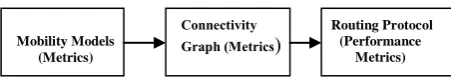
Fig. 6 a relationship among Mobility metrics, Connectivity graph metrics and Routing Protocol performance metrics
Mobility metrics influence connectivity graph which causes effect over routing protocol performance as shown in fig. 6.
3.3.1
Simulation Environment Setup
This section of paper gives simulation work flow and simulation environment setup to evaluate the effect of mobility on the performance of routing protocols. Four mobility models: RWP, RPGM, Manhattan, and Freeway are obtained with generating scenario by setting the parameter of mobility model accordingly in terms of fixed network load as well as varying speed by mobility scenario generator tool and
Mobility Models (Metrics)
Connectivity Graph (Metrics)
Routing Protocol (Performance
[image:4.595.316.542.573.612.2]considered for performance analysis of two on-demand (AODV, DSR) routing protocols in the present work. NS 2.34 is taken as a specific tool, due to its open source code base and specific protocol IEEE 802.11b. Fig. 7 shows simulation environment setup for impact analysis of mobility models on performance of routing protocols.
Fig. 7 Simulation Environment Setup
The objective of analysis is to observe how the routing protocols performance affected with different mobility pattern in fixed network size of 40 nodes and varying node speed 1,5,10,29,30,40,50,60 (m/sec) with 900s simulation time in mobile adhoc environment. A „cbr‟ data packet application of size 512 bytes is taken. The simulation is carried out in region of 1000m x 1000m in present analysis.
3.3.2
Analysis of AODV Performance Metrics
with Different Mobility Patterns
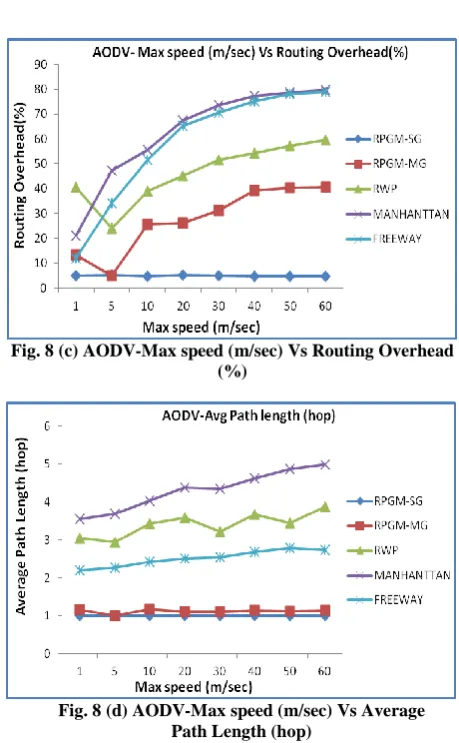
It has been observed that AODV has higher throughput and lower overhead for RPGM-SG, RPGM-MG than other mobility model like RWP, Manhattan and Freeway, haslower average end-to-end delay for RPGM-SG, RPGM-MG than RWP, Manhattan and Freeway and it also has lower average path length (hop count) for RPGM-SG, RPGM-MG than RWP, Freeway, Manhattan, from the analysis and shown in fig. 8 (a-d).
Fig. 8 (a) AODV-Max speed (m/sec) Vs PDF (%)
Fig. 8 (b) AODV-Max speed (m/sec) Vs Average End-End Delay (ms)
Fig. 8 (c) AODV-Max speed (m/sec) Vs Routing Overhead (%)
Fig. 8 (d) AODV-Max speed (m/sec) Vs Average Path Length (hop)
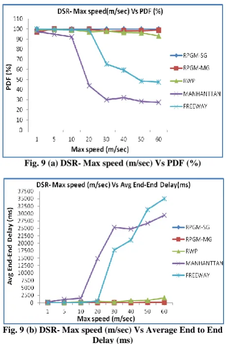
3.3.2- Analysis of DSR Performance Metrics with
Different Mobility pattern
[image:5.595.314.545.77.454.2] [image:5.595.53.283.144.365.2] [image:5.595.313.543.245.617.2] [image:5.595.54.283.580.728.2]Fig. 9 (a) DSR- Max speed (m/sec) Vs PDF (%)
Fig. 9 (b) DSR- Max speed (m/sec) Vs Average End to End Delay (ms)
Fig. 9 (c) DSR- Max speed (m/sec) Vs Routing Overhead (%)
Fig. 9 (d) DSR-Max speed (m/sec) Vs Average Path Length (hop)
4. IMPACT OF MOBILITY PATTERNS
ON BUILDING BLOCKS OF ROUTING
PROTOCOLS
The mechanism of several MANET routing protocols is composed of two major phases-
Route setup phase Route Maintenance phase
4.1 Route Setup Phase
Objective of this phase is for route discovery, if there is no cached route available to the destination. There are two major mechanisms are used to achieve this objective.
First mechanism, called global flooding building block is implemented to distribute the route request messages within the network. The range of flooding is described by TTL field in the IP header. If TTL is set network diameter i.e. TTL=D, a global flooding done. There must be localized controlled flooding before global flooding because it leads high probability of finding an appropriate cache in the neighbourhood.
Second mechanism, called caching building block useful to cache routing information at the nodes, including how to add, invalidate and utilize the cached route entries. It helps to efficiently and promptly provide the route to destination without referring to destination every time. A key parameter i.e. aggressive caching whether it is allowed or not. In general aggressive cache increases the possibility of finding appropriate route without re-initiating route discovery.
Flooding: it is first mechanism as earlier discussed, from simulation, it is observed that number of send route request (RREQ) increases as the mobility increases Vmax shown in from fig. 9 (a-b) for AODV similar to mobility metrics i.e. average relative speed (m/ sec).
AODV: In AODV, fig. 10 (a) shows number of sending route request (RREQ) varying with the node speed. As a standard property, if density of nodes becomes high, the number of sending packets increases in proportion to node density. Simulation shows that low speed mobility generates lower sending route request RREQ than high speed mobility.
[image:6.595.52.282.68.417.2] [image:6.595.52.284.72.772.2] [image:6.595.52.282.411.745.2] [image:6.595.313.542.565.709.2]Fig. 10 (b)AODV- Receive Request (RREQ) for route setup Vs Max speed (m/sec) for various mobility patterns
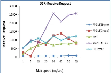
It is observed from fig. 10 (a) that sending route request (RREQ) increases from RWP to Freeway to Manhattan and fig. 10 (b) shows receiving route request (RREQ) increases from RWP to Manhattan to Freeway. It is only because of geographical constraints on movement pattern which turn greater than RWP. Thus, the likelihood of finding a route to destination from source neighbor increases from RWP to Freeway to Manhattan. RPGM (single & 4-group) has a high degree of spatial dependence as shown in fig. 3, which causes high expectation but it is not happen. fig. 10 (a) shows sending route request RREQ lowest for RPGM (single group) than RPGM (4-group). Since, propagating route requests make up large percentage of total route requests in RPGM. These propagating route requests are issued when source sets up a connection to destination for first time. Since, route remains stable for long periods of time, very few route requests retries are done by source.
The number of receiving route request (RREQ) is 10 times larger shown in fig. 10 (b) than shows the number of sending route request (RREQ) in fig. 10 (a). The receiving route request (RREQ) increases as node speed increases than low node‟s mobility as shown in fig. 10 (b).
DSR: Fig. 11 (a-b) shows DSR send request (RREQ) and receive route (RREQ) increased with varying node speed. It is observed in simulation that flooding of RREQ for DSR is low as comparison to AODV during route setup phase which results better performance of DSR than AODV.
Fig. 11 (a) DSR- Send Request (RREQ) for route setup Vs Max speed (m/sec) for various mobility patterns
Fig. 11 (b) DSR- Receive Request (RREQ) for route setup Vs Max speed (m/sec) for various mobility patterns
Since, DSR uses aggressive caching scheme as compared to AODV, therefore, as fig. 9 (a) and fig. 9 (c) of this paper shows that DSR has high throughput and low overhead up to a scalable network size (i.e. 40 nodes) of RWP model. But as network density increases the DSR performance decreases and AODV protocol behaves more effectively to establish the path than DSR protocol over every density. Fig. 11 (a-b) shows sending route request (RREQ) and receiving route (RREQ) lowest value for RPGM (single group) than RPGM (4-group) as compared to rest others mobility models. The number of receiving request (RREQ) is 10 times larger than sending request (RREQ) as shown in fig. 11 (b).
Caching: Caching building block helps to efficiently and promptly provide route to destination without referring to destination every time. There are several parameters affect the behaviour of caching building block. One parameter is whether aggressive caching or multiple caches are allowed. Aggressive caching scheme increases possibility of finding an appropriate route without re-initiating route discovery. DSR uses aggressive caching while AODV do not.
Fig. 12 (a) AODV- Send Route Reply (RREP) for route setup Vs Max speed (m/sec)
[image:7.595.53.281.71.223.2] [image:7.595.315.546.72.224.2] [image:7.595.315.543.485.638.2] [image:7.595.53.281.577.722.2]respectively than other mobility models and effect of mobility is also accordingly. Although, for RWP, Freeway and Manhattan RREP as the node speed increases respectively, it increases disconnection. As node density increases number of RREP packets increases because of dense networks creates path with long hop count as shown in fig. 8 (d). Hop count value is small for group mobility model rather than others. These simulation results conclude that mobility pattern affects connectivity metrics and results flood of route reply (RREP) which will degrade the performance of protocols.
Fig. 12 (b) AODV-Receive Route Reply (RREP) for route setup Vs Max speed (m/sec)
Fig. 13 (a) DSR- Send Route Reply (RREP) for route setup Vs Max speed (m/sec)
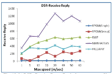
Fig. 13 (b) DSR- Receive Route Reply for route setup Vs Max speed (m/sec)
From fig. 13 (a-b), DSR send route reply (RREP) for route setup is high for Manhattan, RWP and freeway mobility
patterns which imply that most of route replies for these patterns come from cache. Send route replies (RREP) and receives route reply (RREP) increases RPGM (single and 4-group) to Freeway to RWP to Manhattan in the simulation. It shows that caching has adverse effects on mobility patterns with high relative speed and leads invalidation. Packets may be sent on invalid route which might be dropped and leads it retries mechanism, therefore, it results for lower throughput and higher overhead as node density increases for DSR in Manhattan, freeway and RWP mobility pattern in this observation.
It is observed from the simulation, at the higher speed and dense network , number of packets drop or route broken is higher. Therefore ,protocols requires a good error handling mechanism at heigher relative speed or dense network for better performance. Route maintenace is an important building block for detecting broken links and repairing analogous route. Route Maintenance Phase is considered in this paper for detailed description and evaluation.
4.2 Route Maintenance Phase
Mobile Adhoc Network is highly sensitive to some constraints like mobility, bandwidth and wireless propagation losses, therefore, these constraints results unstable links within networks. The unstable links are dealt with in Route Maintenance. Its responsibility is detecting broken links and repairing analogous route. Route maintenance phase has three building blocks:
Error Detection Error Handling Error Notification
Error detection: This building block monitors link status of node with its intermediate nodes. There are several methods to monitor status of node link with its intermediate nodes like MAC level acknowledgements, network layer explicit hello messages or network layer passive overhearing scheme. In this analysis mode of error detection is used.
Error handling: Error handling is a method in which after error detection, a process has been take place for maintenance of broken link with alternate path. There is two way to handle errors:
o Localized Error Recovery
o Non-localized Error Recovery
o Localized Error Recovery: In localized error recovery, node detects broken link and attempts to find an alternative route in its own cache or do a localized flooding before asking source to re-initiate route discovery.
o Non-localized Error Recovery: In non-localized error recovery, node detects link breakage which notify source to handle the error. The source will re-initiate the route discovery procedure if route is still needed.
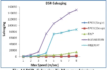
[image:8.595.54.282.186.324.2] [image:8.595.52.281.360.517.2] [image:8.595.52.282.554.707.2]Fig. 14 DSR- Salvaging Vs Max speed (m/sec)
Packet Salvaging:Packet salvaging occurs if an intermediate node forwarding a data packet detects that link to next node is broken. It has another valid route to destination in its route cache. Otherwise, node drops data packet. In all cases, node sends back a RERR packet toward source node. DSR packet salvaging is increases from RPGM (group) to RWP to Freeway to Manhattan and in case of RPGM (Single), it has zero as shown in fig. 14.
Fig. 15 (a) AODV- Send Error Vs Max speed (m/sec)
Fig. 15 (b) AODV- Receive Error Vs Max speed (m/sec)
Send Error and Received Error: In AODV, Hello message is used to monitor link status. If a broken link is detected, a localized route discovery mechanism is re-initiated by upstream node to repair broken route in some scenarios. Nodes within network are notified about error as shown in fig. 15 (a-b).
DSR monitors link status at MAC layer, if a link is broken and detected then salvaging mechanism is used to get alternate
route and at same time a route error message is sent to source for elimination of invalid cache entry. Salvaging is more from RPGM (single & 4-group) to RWP to Freeway to Manhattan in the simulation shown in fig. 14. Although, this building block is good for establishing a new route and helps for performance enhancement but when density of network and node speed increases, it become tougher to manage, therefore protocol performance decreases. This is because DSR performance decreases as compared to AODV protocols.
Localized error handling is initiated in this analysis and number of send error and received error are evaluated for AODV. Send error increases from RPGM (single & 4-group) to RWP to Freeway to Manhattan and number of received error increases from RPGM (single & 4-group) to RWP to Manhattan to Freeway are observed.
[image:9.595.315.542.295.444.2]Nested Error: An analysis of DSR- nested error is carried out, these analysis are shown in fig. 16 with increasing node speed.
Fig. 16 DSR- Nested Errors Vs Max speed (m/sec)
The nested error has been dumped shown for DSR is high for Freeway and Manhattan mobility patterns as node speed increases which cause the performance metrics degradation. Although, it is observed very less nesting error dumped in case of RWP but it has been visualized when the node speed from 50 m/sec in simulation of RPGM (single & 4-group) mobility pattern dumping of nested error is zero in present analysis which shows that the performance of DSR metrics is better than rest of mobility model as shown in fig. 8 (a) and fig. 8 (c) of this paper.
Fig. 17 DSR- Source_SendFailure Vs Max speed (m/sec)
[image:9.595.53.284.326.649.2] [image:9.595.315.543.582.728.2]RWP to Freeway to Manhattan and leads performance degradation accordingly shown in fig. 17.
5. CONCLUSION AND FUTURE WORK
The present work is inclined systematically to analyze the impact of mobility patterns on routing protocols performance of mobile adhoc network. From this analysis, it is observed that mobility pattern influences performance of MANET routing protocols and conclusion is steady with the scrutiny that different mobility patterns have effect on different performance metrics values of protocols. In this investigation; no clear ranking is obtained regarding routing protocols. Analysis shows, impact of mobility models on routing protocols building blocks are influenced, which results routing protocols performance degradation.The scope for future work will lead for proactive protocols (i.e. DSDV, OLSR) over the same considered mobility movement patterns as a next study work.
6. REFERENCE
[1]G.S. Lauer 1995, Packet-radio routing, in: Routing in Communications Networks, ed. M.E. Steenstrup (Prentice Hall) chapter 11, pp. 351–396.
[2]S. Ramanathan and M.E. Steenstrup 1996, A survey of routing techniques for mobile communications networks, Mobile Networks and Applications 98–104.
[3]F. Bai, A. Helmy 2004, “A Survey of Mobility Modeling and Analysis in Wireless Adhoc Networks” in Wireless Ad Hoc and Sensor Networks, Kluwer Academic Publishers.
[4]Nils Aschenbruck, Elmar Gerhards-Padilla, and Peter Martini 2008,” A survey on mobility models for performance analysis in tactical mobile networks”, JTIT, pp: 54-61.
[5]N. Aschenbruck, E. Gerhards-Padilla, M. Gerharz, M. Frank, and P. Martini 2007, “Modelling mobility in disaster area scenarios”, in Proc.10th ACM IEEE Int. Symp. Model. Anal. Simul. Wirel. Mob. Syst.MSWIM, Chania, Greece.
[6]F. Bai, N. Sadagopan, and A. Helmy 2003, “IMPORTANT: a framework to systematically analyze the impact of mobility on performance of routing protocols for adhoc networks”, in Proc. IEEE INFOCOM, San Francisco, USA, pp. 825–835.
[7]Santosh Kumar, S. C. Sharma, Bhupendra Suman 2010,” Mobility Metrics Based Classification & Analysis of Mobility Model for Tactical Network”, International journal of next- generation networks (IJNGN) Vol.2 (3), pp.39-51.
[8]C. Bettstetter, G. Resta, and P. Santi 2003, “The node distribution of the random waypoint mobility model for
wireless ad hoc networks”, IEEE Trans. Mob. Comp., vol. 2(3), pp. 257–269.
[9]C. Bettstetter and C. Wagner 2002, “The spatial node distribution of the random waypoint mobility model”, in Proc. 1st German Worksh. Mob. Ad-Hoc Netw. WMAN’02, Ulm, Germany, pp. 41–58.
[10]C. Perkins, “Ad hoc on demand distance vector (AODV) routing, internet draft, draft-ietf-manet-aodv-00.txt.”
[11]C. E. Perkins and P. Bhagwat 1994, “Highly dynamic destination sequenced distance vector routing (DSDV) for mobile computers,” in ACM SIGCOMM, pp. 234– 244.
[12]J. Broch, D. A. Maltz, D. B. Johnson, Y.-C. Hu, and J. Jetcheva 1998, “A performance comparison of multi-hop wireless ad hoc network routing protocols,” in Proceedings of the Fourth Annual ACM/IEEE International Conference on Mobile Computing and Networking, ACM.
[13]D. B. Johnson, D. A. Maltz, and J. Broch 2001, “”DSR: The dynamic source routing protocol for multi-hop wireless ad hoc networks”,” in Ad Hoc Networking, C. Perkins, Ed. Addison-Wesley, pp. 139–172.
[14]X. Hong, M. Gerla, G. Pei, and C.-C. Chiang 1999, “A group mobility model for ad hoc wireless networks,” in ACM/IEEE MSWiM.
[15]Qunwei Zheng, Xiaoyan Hong, and Sibabrata Ray 2004,” Recent Advances in Mobility Modeling for Mobile Ad Hoc”, In ACMSE’04, Huntsville, Alabama, USA Copyright 2004 ACM 1581138709/04/04.
[16]P. Johansson, T. Larsson, N. Hedman, B. Mielczarek, and M. germark 1999,“Scenario-based performance analysis of routing protocols for mobile ad-hoc networks,” in International Conference on Mobile Computing and Networking (MobiCom’99), pp. 195–206.
[17]Fan Bai, Narayanan Sadagopan, Ahmed Helmy 2004, “User Manual for Important Mobility Tool Generators in NS-2 Simulators”.
[18]M. Musolesi and C. Mascolo 2008, “Mobility Models for Systems Evaluation,” in MINEMA: Proceedings of the Workshop State of the Art on Middleware for Network Eccentric and Mobile Applications, Glasgow, Scotland,Great Britain.
[19]S. Bittner, W.-U. Raffel and M. Scholz 2005, “The area graph-based mobility model and its impact on data dissemination”, in Proc. IEEE PerCom, Kuaai Island, Hawaii, USA, pp. 268–272.