SPC for Software Reliability
using Inflection S-Shaped Model
R.Satya Prasad,
PhD. Associate Professor Dept.of Computer Science & Engg.,Achrya Nagarjuna University Guntur
Y.Sangeetha
Asst.ProfessorDept.of Information Technology V.R.Siddhartha Engg.College
Vijayawada
ABSTRACT
Traditional statistical analysis methods account for natural va-riation but require aggregation of measurements over time,which can delay decision making.Statistical process con-trol (SPC) is a branch of statistics that combines rigorous time series analysis methods with graphical presentation of data,often yielding insights into the data more quickly and in a way more understandble to lay decision makers .SPC and its primary tool-the control chart-provide researchers and practi-tioners with a method of better understanding and communica-ting data from software reliability improvement process efforts .This paper provides an s-shaped software reliability growth model based on the Non-Homogenous Poisson Process (NHPP).The maximum likelihood approach is used to esti-mate the unknown parameters of the model.
Keywords: Statistical Process Control, software reliability, mean value function, probability limits, control charts, Inflec-tion s-shaped.
1 INTRODUCTION
Software reliability is a key part in software quality. The study of software reliability can be categorized into three parts: mod-eling, measurement and improvement. Software reli-ability modeling has matured to the point that meaningful re-sults can be obtained by applying suitable models to the prob-lem. There are many models that exist, but no single model can capture a necessary amount of the software characteristics. Assumptions and abstractions must be made to simplify the problem. There is no single model that is universal to all the situations. Software reliability cannot be directly measured, so other related factors are measured to estimate software relia-bility and compare it among products. Development process, faults and failures found are all factors related to software relia-bility. Software reliability improvement is complex process. The difficulty of the problem stems from insufficient under-standing of software reliability and in general, the characteris-tics of software. Until now there is no good way to conquer the complexity problem of software the difficulty of the problem stems from insufficient understanding of software reliabil-ity.The difficulty of the problem stems from insufficient under-standing of software reliability and in general, the characteris-tics of software. Until now there is no good way to conquer the complexity problem of software. Defect-free software product cannot be assured. Realistic constraints of time and budget severely limit the effort put into software reliability improve-ment. Software quality and reliability must be made to simplify the problem. There is no single model that is universal to all the situations. Software reliability cannot be directly meas-ured, so other related factors are measured to estimate soft-ware reliability and compare it among products.
Software quality and reliability can be achieved by eliminating the causes or improving the software process or its operating procedures [2].Applying statistical process control (use of con-trol charts) to the management of software development efforts, to effect software process improvement. Deploying Statistical Process Control is a process in itself, requiring organi-zational commitment across functional boundaries. SPC proce-dures can help you monitor process behavior [13]. The SPC chart selection is based on data, situation and need [4].Control charts are an efficient way of analyzing per-formance data in order to evaluate a process. A control chart is a popular statistical tool for monitoring the quality of goods and services, and for detecting when the process goes “out of con-trol” as early as possible. The data from measurements of varia-tions at points on the process map is monitored using control charts. Using control charts is a continuous activity, ongoing over time. Considering above, software reliability measurement is a complex process which needs rational reliability models.
2 NHPP MODEL
The Non-Homogenous Poisson Process (NHPP) based software reliability growth models (SRGMs) are proven to be quite suc-cessful in practical software reliability engineering [1, 3,12]. The main issue in the NHPP model is to determine an appropri-ate mean value function to denote the expected number of fail-ures experienced up to a certain time point. Model parameters can be estimated by using Maximum Likelihood Estimate (MLE).
Let
N
t
,
t
0
be the cumulative number of software failures by time‘t’. m(t) is the mean value function, representing the expected number of software failures by time ‘t’.
t
Is the failure intensity function, which is proportional to there-sidual fault content. Thus
m
t
a
(
1
e
bt)
and
(
)
b
(
a
m
(
t
))
dt
t
dm
t
. where ‘a’ denotes theini-tial number of faults contained in a program and ‘b’
represents the fault detection rate. In software reliability, the initial number of faults and the fault detection rate are al-ways unknown. The maximum likelihood technique can be used to evaluate the unknown parameters. In a more
general NHPP SRGM
t
can be expressed as
b
t
a
t
m
t
dt
t
dm
t
(
)
. Wherea
t
is theand introduced faults in the program and
b
t
is the time-dependent fault detection rate.3 MODEL DESCRIPTION: INFLECTION
S-SHAPED MODEL
Software reliability growth models have been grouped into two classes of models concave and S-shaped. The most important thing about both models is that they have the same as-ymptotic behavior, i.e., the defect detection rate decreases as the number of defects detected (and repaired) increases, and the total number of defects detected asymptotically approaches a finite value. The inflection S-shaped model was proposed by [5,6]. This model assumes that the fault detection rate increases throughout a test period. The model has a parameter, called the inflection rate, which indicates the ratio of detectable faults to the total number of faults in the target software. True, sustained exponential growth cannot exist in the real world. Eventually all exponential, amplifying processes will uncover underlying stabilizing processes that act as limits to growth. The shift from exponential to asymptotic growth is known as sigmoidal, or S-shaped, growth.
Ohba models the dependency of faults by postulating the following assumptions:
Some of the faults are not detectable be-fore some other faults are removed.
The detection rate is proportional to the number of detectable faults in the program.
Failure rate of each detectable fault is constant and identical.
All faults can be removed.
Assuming [7]:
bte
b
t
b
1
This model is characterized by the following mean value
func-tion:
bt
bt
e
e
a
t
m
1
1
)
(
Where ‘b’ is the failure detection rate, and ‘
’ is the inflec-tion factor. The failure intensity funcinflec-tion is given as:
21
1
)
(
bt bte
abe
t
4 PARAMETER ESTIMATION: MLE
The idea behind maximum likelihood parameter estimation is to determine the parameters that maximize the probability (likelihood) of the sample data. The method of maximum like-lihood is considered to be more robust (with some exceptions) and yields estimators with good statistical properties. In other words, MLE methods are versatile and apply to most models and to different types of data. Although the
methodolo-gy for maximum likelihood estimation is simple, the implementation is mathematically intense. Using today's
com-puter power, however, mathematical complexity is not a big obstacle. Conduct an experiment and obtain N independent
observations,
1
, ,
2,
Nt t
t
. Then the likelihood function [9] is given by the following product:
N i k i kN
L
f
t
t
t
t
L
1 2 1 2 1 21
,
,
,
|
,
,
,
(
;
,
,
,
)
Likely hood function by using λ(t) is: L =
n i it
1)
(
The logarithmic likelihood function is givenby:
N i k it
f
L
1 21
,
,
,
)
;
(
ln
ln
LogLikeli-hood function is: Log L = log (
n i it
1)
(
)Which can be written [10] as
1
1 1.log ( ) ( )
n
i i i i n
i
y y m t m t m t
The maximum likelihood estimators (MLE) of
1,
2,
,
k are obtained by maximizing L or
, where
is in L. By max-imizing , which is much easier to work with than L, themax-imum likelihood estimators (MLE) of
1,
2,
,
kare the simultaneous solutions of k equations such that:
0
j
, j=1,2,…,kThe parameters ‘a’ and ‘b’ are estimated using iterative Newton
Raphson Method, which is given as
)
(
'
)
(
1 n n n nx
f
x
f
x
x
5 ILLUSTRATING THE MLE METHOD
PARAMETER ESTIMATION
To estimate ‘a’ and ‘b’, for a sample of n units, first obtain the
likelihood function: assuming
0
.
05
.
N i bt bte
abe
L
1 21
1
Take the natural logarithm on both sides, The Log Likelihood
function is given as:
Log L =
log[
(
)
]
=
n i bt bte
abe
1 21
1
log[
n i bt bt bt bte
e
a
e
abe
1 21
1
)
1
1
log(
Taking the Partial derivative w.r.t ‘a’ and equating to ‘0’. (i.e.
0
log
a
L
)a= ……… (5.1)
Taking the Partial derivative w.r.t ‘b’ and equating to ‘0’.(i.e.
0
log
)
(
b
L
b
g
) g(b)=−1 − −11+ − −1-
1 +2 1 1+ ... ...(5.2)
Taking the partial derivative again w.r.t ‘b’ and equating to ‘0’.
(i.e.
'
(
)
log
20
2
b
L
b
g
) g’(b)= - ……….(5.3)The parameter ‘b’ is estimated by iterative Newton Raphson
Method using
)
(
'
)
(
1 n n n nb
g
b
g
b
b
, which is substituted infinding ‘a’.
6 DISTRIBUTION OF FAILURE COUNT
DATA
Based on the failure count data given in Table 1 & 2, we com-pute the software failures process through Mean Value Control chart. We used cumulative Failure count data for software reliability monitoring using inflection s-shaped distribution.
Assuming an acceptable probability of false alarm of 0.27%, the control limits are calculated by solving the fol-lowing equations.
1
0
.
99865
1
1
bt bt Ue
e
T
1
0
.
5
1
1
bt bt Ce
e
T
1
0
.
00135
1
1
[image:3.595.47.556.25.748.2]
bt bt Le
e
T
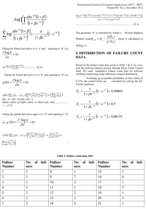
Table 1: Failure count data, DS1
Failure
Number
No. of
fail-ures
Failure
Number
No. of
fail-ures
Failure
Number
No. of
fail-ures
1
2
8
1
15
1
2
1
9
7
16
6
3
1
10
3
17
1
4
1
11
1
18
3
5
2
12
2
19
1
6
2
13
2
20
3
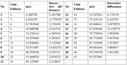
Table 2: Failure count data, DS2
Failure
Number
No. of
fail-ures
Failure
Number
No. of
fail-ures
Failure
Number
No. of
fail-ures
1
6
8
3
15
5
2
2
9
2
16
2
3
1
10
3
17
2
4
1
11
1
18
2
5
3
12
3
19
1
6
1
13
2
20
3
7
2
14
5
‘a’ and ‘
b’ are Maximum Likely hood Estimates (MLEs) of parameters and the values can be computed using iterative method for the given cumulative time between failures data shown in Table 1 & 2. Using ‘a’ and ‘b’ values we can compute
m
(
t
)
.These limits are converted to
m
(
t
U)
,m
(
t
C)
and)
(
t
Lm
form. They are used to find whether the softwarepro-cess is in control or not by placing the points in Mean value chart shown in figure 1 & 2. A point below the control limit
)
(
t
Lm
indicates an alarming signal. A point above the controllimit
m
(
t
U)
indicates better quality. If the points are falling within the control limits it indicates the software process is in stable[8].
Table 3: Estimated parameters and the corresponding control limits
Data set
A
b
m(t
u)
m(t
c)
m(t
l)
DS1
871.823132
0.002646
869.880070
435.878051
1.176445
DS2
2664.972820 0.000874
2660.57464
1332.21952
3.59737
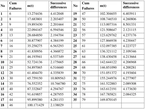
Table 4: DS1-Successive differences of cumulative mean values.
No
Cum
Failures
m(t)
Succes-sive
dif-ferences
No
Cum
Failures
m(t)
Successive
differences
1
2
4.380758
2.181700
12
25
53.255941
4.179178
2
3
6.562459
2.1759357
13
27
57.435119
8.165291
3
4
8.7383948
2.170185
14
31
65.600411
2.0278552
4
5
10.908580
4.341534
15
32
67.628266
12.150753
5
7
15.250114
4.305545
16
38
79.779019
1.993030
6
9
19.555660
4.282821
17
39
81.772050
5.947548
7
11
23.838481
2.132926
18
42
87.719598
1.972047
8
12
25.971407
14.822531
19
43
89.691646
5.884931
9
19
40.793938
6.255731
20
46
95.576578
1.951285
10
22
47.049670
2.074233
21
47
97.527863
Table 5: DS2-Successive differences of cumulative mean values.
No
Cum
Failures
m(t)
Successive
differences
No
Cum
Failures
m(t)
Successive
differences
1
6
13.274436
4.412048
19
47
102.304655
6.403911
2
8
17.683801
2.203407
20
50
108.746510
4.260806
3
9
19.893430
2.201664
21
52
113.007316
8.501331
4
10
22.094167
6.594546
22
56
121.508647
2.121115
5
13
28.684850
2.194704
23
57
123.629762
4.237176
6
14
30.877907
4.384199
24
59
127.866938
4.230447
7
16
35.258275
6.563293
25
61
132.097385
4.223727
8
19
41.830956
4.366872
26
63
136.321112
2.109346
9
21
46.193941
6.537349
27
64
138.430458
4.213664
10
24
52.724136
2.175665
28
66
142.644122
4.206968
11
25
54.897065
6.516660
29
68
146.851090
4.200281
12
28
61.404470
4.335839
30
70
151.051372
4.193604
13
30
65.759150
10.809563
31
72
155.244976
6.277907
14
35
76.552352
10.766780
32
75
161.522883
2.089308
15
40
87.332847
4.294767
33
76
163.612191
4.173630
16
42
91.619857
4.287955
34
78
167.785821
2.084325
17
44
95.899380
4.281153
35
79
169.870145
18
46
100.171429
2.138029
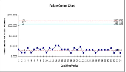
By placing the differences of cumulative failure counts shown in table 4 and 5 on y axis, failure number on x axis and the values of control limits being placed on Mean Val-ue chart, we obtained figure 1 & 2. The first Mean ValVal-ue chart shows that all the mean value successive differences are within the control limits, which indicates that the process is in
stable state. Whereas the in the second chart some of the suc-cessive differences are out of control limits, which indicates the failure process is identified. It is significantly early detection of failures using Mean Value Chart [11]. The software quality is determined by detecting failures at an early stage.
Figure: 1 Mean Value Chart for DS1
mean value chart
UCL 869.8800709
CL 435.878051601
LCL 1.176445761
0.100000000 1.000000000 10.000000000 100.000000000 1000.000000000
1 2 3 4 5 6 7 8 9 10 11 12 13 14 15 16 17 18 19 20
Date/Time/Period
suc
ce
ss
iv
e
di
ff
er
enc
[image:5.595.55.554.550.742.2]Failure Control Chart
UCL
2660.5746
CL
1332.2195
LCL
3.5974
1.0000
10.0000
100.0000
1000.0000
10000.0000
1 2 3 4 5 6 7 8 9 10 11 12 13 14 15 16 17 18 19 20 21 22 23 24 25 26 27 28 29 30 31 32 33 34
Date/Time/Period
di
ff
e
r
e
nc
e
s
of
m
e
a
n
v
a
lue
s
[image:6.595.92.535.80.334.2]
Figure: 2 Mean Value Chart for DS2
7 CONCLUSION
The successive differences of failure counts are plotted through the estimated mean value function against the failure serial order. The parameter estimation is carried out by New-ton Raphson Iterative method for inflection s-shaped model. The graph of data set DS1 in figure 1 has shown all the points with in control limits .By observing the Mean Value Control chart of data set DS2,it is identified that failure situation is detected at 2nd point ,which is below m .It indicates that the failure process is detected at an early stage. Hence we conclude that our method of estimation and control chart are giving a positive recommendation for their use in finding out preferable control process or desirable out of control signal .The early detection of software failure will improve the soft-ware reliability.
8 REFERENCE
[1] Geetha Rani, N., Satya Prasad, R., & Kantham, R.R.L., (2011).Software Reliability Growth Model Using Inter-val Domain Data. International Journal of Computer Applications, Vol 34[9], Pp.5-8.
[2] Kimura, M., Yamada, S., Osaki, S., (1995).Statistical Software Reliability prediction and Its Applicability Based on Mean Time Between Failures. Mathematical and Computer Modeling, Vol 22, Issues 10-12, Pp. 149-155.
[3] Krishna Mohan G., & Satya Prasad, R., (2011). Interval Domain Based Software Process Control Using Weibull Mean Value Function. International Journal of Computer Science and Information Technology and Security, Vol 1[2], Pp.111-114.
[4] Macgregor, J.F., Kourti, T., (1995).Statistical Process Control of Multivariate Processs.Control Engineering Practice, Vol 3, Issue 3, Pp.403-414, Canada: Elsevier. [5] Ohba, M., (1984). Software Reliability Analysis Model.
IBM J. Res. Develop, Vol 28, Pp.428-443.
[6] Ohba, M., (1984a). Software Reliability Analysis Mod-els. IBM Journal Research Development, Vol.21 (4).
[7] Ohba, M., & Yamada, S., (1984b). S-Shaped Software Reliability Growth Models .Proc.4thInt.Conf.Reliabilit and Maintainability, Pp.430-436.
[8] Pham. H., (1993). Software Reliability Assessment: Im-perfect Debugging and Multiple Failure types Software Development. EG&GRAAM-10737, Salt Lake: Idaho National Engineering Laboratory.
[9] Pham. H., (2003). Handbook of Reliability Engineering, London: Springer.
[10] Pham. H., (2006). System software reliability, Lon-don: Springer.
[12] Satya Prasad, R., Gotham, V., & Krishna Mohan G., (2011). Interval Domain Software Process Control – Goelokumoto. International Journal of Research and Reviews in Computer Science, Vol 2[4], Pp.1001-1004. [13] Xie, M., Goh. T.N., & Ranjan, P., (2002). Some