A Fast Approach to Clustering Datasets using DBSCAN
and Pruning Algorithms
S.Vijayalaksmi
Research and development centre, Bharathiar University,
Coimbatore
M Punithavalli, PhD.
Director, MCA Dept. Sri Ramakrishna Engg.CollelgeCoimbatore
ABSTRACT
A
mong the various clustering algorithms, DBSCAN is an effective clustering algorithm used in many applications. It has various advantages like no a priori assumption needed about the number of clusters, can find arbitrarily shaped clusters and can perform well even in the presence of outliers. However, the performance is seriously affected when the dataset size becomes large. Moreover, the selection of the two input parameters, Eps and MinPts, has a great impact on the clustering performance. To solve these two problems, this paper modifies the traditional DBSCAN algorithm in two manners. The first method uses K-dimensional tree instead of the traditional R-tree algorithm while the second method includes a locally sensitive hash procedure to speed up the process of clustering and increase the efficiency of clustering. The algorithms use a k-distance graph method to automatically calculate Eps and MinPts. Experimental results show that both the algorithms are efficient in terms of scalability and speeds up the clustering process in an efficient manner.Keywords: DBSCAN, Speed Optimization, Nearest Neighbour Search, KD-Tree, Locally Sensitive Hashing.
1. INTRODUCTION
The beginning of the twenty first century has brought considerable advances in the field of computer-based information retrieval systems, where data with “hidden asset” called “knowledge” is quickly becoming the most valuable resource. The current era of information explosion utilizes powerful data mining techniques that can efficiently analyze, interpret and extract valuable knowledge. The rapid growth in the number and size of databases, dimension and complexity of data has made it necessary to automate the analysis process, whose results can then be used by decision-making processes. Data mining is a multi-faceted area which uses a variety of data analysis tools to discover patterns and relationships in data.
Clustering and classification are two popular data mining techniques [14]. The popularity is behind the fact that they are the first data mining techniques to examine the structure and patterns in data.
Clustering analysis partition data objects objectively based on measuring the mutual similarity between data objects. It is a method that divides a set of objects into subsets, called clusters, such that the objects in any cluster are similar to those inside it and different from those outside it [13].Clustering has a long and rich history in a variety of scientific fields like image segmentation, information retrieval and web data mining. Clustering algorithms can be
categorized into partition-based algorithms [16], hierarchical-based algorithms spectral algorithms, density-hierarchical-based algorithms [8]and grid-based algorithms [3] These methods vary in (i) the procedures used for measuring the similarity (within and between clusters) (ii) the use of thresholds in constructing clusters (iii) the manner of clustering, that is, whether they allow objects to belong to strictly to one cluster or can belong to more clusters in different degrees and the structure of the algorithm. Irrespective of the method used, the resulting cluster structure is used as a result in itself, for inspection by a user, or to support retrieval of objects
Among these, density-based algorithms have gained much interest in the research community; [10] DBSCAN (Density-Based Spatial Clustering of Applications with Noise), a density based clustering algorithm is an effective clustering algorithm for Spatial Database Systems. It has the following advantages.
1. DBSCAN does not require knowing the number of clusters in the data a priori, as opposed to k-means.
2. DBSCAN can find arbitrarily shaped clusters.
3. Performance does not degrade with the presence of outliers
DBSCAN requires just two parameters and is mostly insensitive to the ordering of the points in the database. However, the algorithm also has some issues with regard to execution time and its time complexity is O(n log n) The algorithm fails to scale well to large dimensions because of this complexity that mainly arises because of the searching the neighbourhood process. In this paper, two techniques are proposed to solve this problem and improve the speed of DBSCAN clustering. The first method aims to reduce the time required to search the neighbourhood by using an efficient tree called kd-tree. The second uses a Locally-Sensitive Hashing method to reduce the neighbourhood search time and thus reduce the overall time requirement for DBSCAN algorithm. The rest of the paper is organized as follows. A brief study of the existing solutions is given in Section 2. Section 3 presents the traditional DBSCA algorithm along with the two proposed time-efficient fast DBSCAN variants. The experimental results are discussed in Section 4 while Section 5 concludes the research work with future research directions.
2. LITERATURE STUDY
Volume 60– No.14, December 2012
technique that reduces the search space and thus indirectly reduces the time required by DBSCAN. Several partitioning algorithms like CLARANS [6], K-Means simple one-pass clustering [15] have been used for this purpose. Space indexing techniques such as R-tree or X-tree have also been used for fast retrieval of an object’s neighbors in a data set, where indexing techniques can be classified as space partitioning methods. In partition based DBSCAN algorithm, partition is considered as a pre-processing step and normally comes with its overheads like requiring extra memory, extra computations and determining the correct values for input parameters. The second method ‘sampling’ involves selecting only a subset of the data set and using DBSCAN on randomly selected subsets to form clusters. Examples include SDBSCAN and Rough-DBSCAN. In these techniques, a tradeoff between sampling rates and speed exists. That is, low sampling rates decreases the time requirement but degrade the clustering accuracy. Reducing the time requirement through smart core detection methods was used by FDBSCANand IDBSCAN [4]. Combining k-means and core point detection methods was performed by KIDBSCAN.
This method first located the high-density areas using k-means algorithm and then introduced core points with respect to density rankings. Similarly core point detection and sampling method was combined by [20] to improve the time requirement of DBSCAN. SPARROW [9] reduces the number of core points using a method that is inspired by the flocking mechanism of birds. Smart detection of core points and sampling on the core points may result in anomalies such as falsely dividing the original clusters and false identification of border points as noise. Parallel approaches of DBSCAN are introduced in [19];[11]. Although parallel implementations may improve the execution time performance locally at each processor, combining the results into the final output is not trivial.
3. PROPOSED FAST VARIANTS OF
DBSCAN
Dbscan algorithm has its own definition. The definition defines that point p is reachable from point p when both the points are falls in the given distance. And point p is consider only when p1,p2,p3 points are so close to it. So a cluster should have the property like density connected points should be part of cluster and all the points should mutually density connected. Dbscan needs two input parameters namely eps and minpts. Eps is the radius of the cluster and minpts is minimum number of points in that cluster. Normally Dbscan starts its journey from arbitrary starting point x which is not visited already. If x has n number of neighbor then each point will be visited and labeled as visited and that points will be accumulated in the clusters. If but x does not have neighbor point and it is not fll in given radius the that particular point will be marked as noise. This is process will continue up to the unvisited point in given distance.
Hence, all points that are found within the ε-neighborhood are added, as is their own ε-ε-neighborhood. This process continues until the cluster is completely found. Then, a new unvisited point is retrieved and processed, leading to the discovery of a further cluster or noise. However, the algorithm also has some major drawbacks which are as follows:
The algorithm has two global parameters “ε” and “MinPts”, estimation of which is difficult for an arbitrary dataset.
The algorithm fails to scale well to large dimensions because of the complexity of searching the neighbourhood in large dimensions
3.1.KD Tree based DBSCAN
(KDT-DBSCAN)
Both the problems are solved in the present work by using an automated process for identifying and MinPts values and using KD-Tree to solve the problem search complexity. The use of kd tree is to segment the data structure for aligning points in k-dimensional space. When there is need to use multidimensional key, there the kd tree plays its role. Kd tree has two nodes and k dimensional points so it called as binary tree.
Every non-leaf node can be thought of as implicitly generating a splitting hyperplane that divides the space into two parts, right and left subspaces. Every node in the tree is associated with one of the k-dimensions, with the hyperplane perpendicular to that dimension's axis. So, for example, if for a particular split the "x" axis is chosen, all points in the subtree with a smaller "x" value than the node will appear in the left subtree and all points with larger "x" value will be in the right sub tree. In such a case, the hyperplane would be set by the x-value of the point, and its normal would be the unit x-axis [2] Given a list of n points, the algorithm given in Figure 2 constructs a balanced k-d tree containing those points.
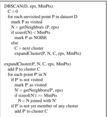
DBSCAN(D, eps, MinPts) C = 0
for each unvisited point P in dataset D mark P as visited
N = getNeighbors (P, eps) if sizeof(N) < MinPts mark P as NOISE else
C = next cluster
expandCluster(P, N, C, eps, MinPts)
expandCluster(P, N, C, eps, MinPts) add P to cluster C
for each point P' in N if P' is not visited mark P' as visited N' = getNeighbors(P', eps) if sizeof(N') >= MinPts N = N joined with N'
if P' is not yet member of any cluster add P' to cluster C
[image:2.595.340.528.406.611.2]
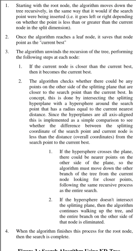
The NN (nearest neighbor) algorithm is used to find the points in the tree which is nearest to a point given. This algorithm is very useful because easily it can avoid large search space. Searching for a nearest neighbour in a k-d tree proceeds is given in Figure 3.
In order to automatically detect the two parameters epsilon and min-pts required by DBSCAN, this section proposed the use of k-distance graph. Let ‘d’ be the distance of a point ‘p’ to its kth nearest neighbor, then the d-neighborhood of ‘p’ contains exactly k+1 points for almost all points ‘p’. The d-neighborhood of ‘p’ contains more than k+1 points only if several points have exactly the same distance ‘d’ from ‘p’ which is quite unlikely. Furthermore, changing ‘k’ for a point in a cluster does not result in large changes of ‘d’. This only happens if the kth nearest neighbors of p for k = 1, 2, 3, are located approximately on a straight line which in general is not true for a point in a cluster.
[image:3.595.59.261.53.232.2]For a given k, a function k-dist from the database D is defined by mapping each point to the distance from its kth nearest neighbor. When sorting the points of the database in descending order of their k-dist values, the graph of this function gives some hints concerning the density distribution in the database. This graph is called the sorted k-dist graph. If an arbitrary point ‘p’ is chosen, set the parameter Eps to k-dist(p) and set the parameter MinPts to k, all points with an equal or smaller k-dist value will be core points. However, as indicated by Ester et al. (1996), the k-dist graphs for k > 4 do not significantly differ from the 4-dist graph and they need considerably more computations. The applicability of value 4 to MinPts was further proved by several proposals [17]; [18]. Therefore, the parameter MinPts is set to 4 during experimentations. The 4-dist value of the threshold point is used as the Eps value for DBSCAN. These estimated values were given as input to the DBSCAN algorithm given in Figure 2
The time requirement of DBSCAN algorithm is O(n log n) where n is the size of the dataset. This when combined with k-distance graph to automatically select MinPts and Eps values, increases to O(n2 log n). Usage of KD Tree (space partitioning tree) reduced the time complexity to O(log n). While using KD-Tree finding k nearest neighbours for each n data point the complexity is O(kn log n). The k value is very negligible and therefore does not make much different and hence the time complexity becomes O(log n).
3.2.LSH-based DBSCAN (LSH-DBSCAN)
Locally Sensitive Hashing (LSH) is an efficient randomized search technique proposed by The k-dist function used to find the kth nearest neighbor of given point. In the k-dist function there is graph called k-graph which has the purpose of finding density distribution of given set of points.. The principle of hash function is to collect the items in the same bucket which are uniform and with high probability.
LSH (Locality sensitive hashing ) is method which accumulate the group of points into a same bucket based on the distance metric. The algorithm is popular in similarity searching [5], malware clustering [1] and hierarchical clustering. An LSH F is defined for a metric space M = (M, d), a threshold R>0 and an approximation factor c > 1. An LSH family F is a family of functions h : m S satisfying
1. Starting with the root node, the algorithm moves down the tree recursively, in the same way that it would if the search point were being inserted (i.e. it goes left or right depending on whether the point is less than or greater than the current node in the split dimension).
2. Once the algorithm reaches a leaf node, it saves that node point as the "current best"
3. The algorithm unwinds the recursion of the tree, performing the following steps at each node:
1. If the current node is closer than the current best, then it becomes the current best.
2. The algorithm checks whether there could be any points on the other side of the splitting plane that are closer to the search point than the current best. In concept, this is done by intersecting the splitting hyperplane with a hypersphere around the search point that has a radius equal to the current nearest distance. Since the hyperplanes are all axis-aligned this is implemented as a simple comparison to see whether the difference between the splitting coordinate of the search point and current node is less than the distance (overall coordinates) from the search point to the current best.
1. If the hypersphere crosses the plane, there could be nearer points on the other side of the plane, so the algorithm must move down the other branch of the tree from the current node looking for closer points, following the same recursive process as the entire search.
2. If the hypersphere doesn't intersect the splitting plane, then the algorithm continues walking up the tree, and the entire branch on the other side of that node is eliminated.
4. When the algorithm finishes this process for the root node, then the search is complete.
Figure 3 : Search Algorithm Using KD-Tree Input : List of points pointList and depth
Output : KD Tree
Function kdtree(pointList, depth)
Step 1 : Select axis based on depth so that axis cycles through all valid values (axis = depth mod k) Step 2 : Sort point list and choose median as pivot
element
Step 3 : Create node and construct subtrees node location := median;
leftChild := kdtree(points in pointList before median, depth+1);
rightChild := kdtree(points in pointList after median, depth+1);
[image:3.595.59.284.335.750.2]Step 4 : Repeat Steps 1 - 3 till pointList in empty.
Volume 60– No.14, December 2012
the following conditions for any two points p, q M and a function h chosen uniformly at random from F:
if d(p, q) R, then h(p) = h(q) (i.e, p and q collide) with probability at least P1.
If d(p, q) cR, then h(p) = h(q) with probability at most P2.
A family is said to be interesting when P1 > P2 and such a family F is called (R, cR, P1, P2)-sensitive.
One of the easiest ways to construct an LSH family is by bit sampling. This approach works for the Hamming distance over d-dimensional vectors {0, 1}d. Here, the family F of hash functions is simply the family of all the projections of points on one of the d coordinates, i.e., F = {h : {0, 1}d {0, 1} | h(x) = xi, i = 1 .. d}, where xi is the ith coordinate of z. A random function h from F simply selects a random bit from the input point. This family has the following parameters P1 = 1- R/d and P2 = 1-cR/d.
In the proposed method is used to reduce the neighbourhood search time. In DBSCAN, the nearest neighbour point search returns all those points inside a circle with center ‘Ce’ and radius ‘ra’. While using with LSH, the nearest neighbour search (NNS) returns only approximate points, that is, it returns only those points of ‘Ce’ with radius (1+)d, where is a user defined value and is > 0. For each point, its retrieval time complexity is O(d log C), where d and C are independent to N and LSH guarantees that the query time is O(D*N1/1+) for approximate nearest neighbor query over an n-point database . The differences between DBSCAN based on the LSH algorithm and the original DBSCAN are as follows.
The LSH algorithm enhances original DBSCAN by substituting its retrieval technique for LSH, improves NNS of DBSCAN by hashing and decreasing time complexity
Being different from original LSH, after obtaining the points retrieved by LSH, wrong points which are far from the center point are removed and thus the scale of the data is reduced.
The algorithm works in two steps. The first step constructs the LSH hash index and the second step uses DBSCAN to cluster the dataset using the index created in the previous step. Let the LSH family be F, the algorithm has two parameters, width (k) and number of hash functions (L). In the first step, a new family G of hash function g is defined, where each function g is obtained by concatenating k randomly chosen hash function from F, i.e., g(p)=[h1(p), …, hk(p)]. In other words, a random hash function g is obtained by concatenating k randomly chosen hash functions from F. The algorithm then constructs L hash tables, each corresponding to a different randomly chosen hash function g.
Initially all n points from a dataset S is hashed into each of the L hash tables. The hashing function is chosen in
such a way that it results with hashing tables that has only n non-zero entries and can reduce the amount of memory used per hash table to O(n). The hash function used in the study is described below. Given an input data X, the hash function selects a random integer d from [1, D], where D is the number of attributes in the dataset and selects random Vid from [a, b] (Equation 1).
id V d X 0
id V d X 1 ) d X ( F
(1)
Using the above equation, for each input data, a k length string which is composed of 0 and 1 can thus be obtained. The hash function exhibits an important property required by NSS algorithms That is, when two data are very similar then the probability of them falling into the same hash table is high and vice versa.
The main concern of using LSH algorithm in NNS is the parameter selection L and K. In this study, an automatic estimation process is used. Given two probabilities, P1 and P2, k and L can be calculated using Equation (2).
2
1/P
log
n
log
K
and L =n where =
log
P
2
1
P
log
(2)
The method used to estimate the two parameters Eps and MinPts is the same as the method described in Section 3.1. The proposed LSH-DBSCAN algorithm is described in Figure 4.
Input: M - the dataset Output: Clusters
Step 1 : Estimate parameters Eps, MinPts, K and L Step 2 : Initialization
Begin
for i from 1 to K do
randomly generate hashing function gi(·) for i from 1 to L do
generate hashing tables Ti
// result of Step 2
Step 3 : Clustering Procedure */
Repeat
while not end of the dataset do
Take out object p in turn from the dataset Validate a query point p using Figure 5 with hash table T, Eps
if p is approximate core object then Take the approximate core point p as the
center
Find all approximate density-connected points and group them into a cluster
Completely deletes them from M. For all appropriate core points in M
Mark the remaining points as noisy clusters (outliers) End
In the above procedure, the valid(p) function is used to remove all dissimilar points and restricts all approximately nearest neighbour points with the Eps radius circle. The procedure is given in Figure 5.
The time and space complexities of the proposed LSH-DBSCAN algorithm depends on the size of dataset (n), the dimension of hash table (K), the number of hash tables (L) and the number of attributes (D). From Step 2 of Figure 4, the time complexity is O(L*K). In the Clustering procedure (Step 3), the time of searching a point p is O(K log C) where log C is a constant. According to Aristides’ experiment, the value of C can be made very small and can be ignored. Thus, the time complexity of this step becomes O(K). For the whole dataset, the time complexity is then O(N*K).
During clustering, the algorithm needs to store L hash tables and the dataset in the main memory, so the space complexity of the proposed LSH-DBSCAN is O(K*L+N*D), while the traditional algorithm required O(N*D). Obviously, the space complexity of both algorithms can be deemed as O(N). The above analysis shows that, comparing with the former algorithms, the improved DBSCAN algorithm can reduce the time complexity without increasing the space complexity.
4.EXPERIMENTAL RESULTS
The effectiveness of the proposed clustering algorithms was evaluated using various datasets and performance metrics. Both small and large sized real-life datasets were used during experimentation. The real-life datasets were obtained from UCI Machine Learning Repository[12] and the numeric attributes were normalized according to a normal distribution and categorical values were converted to an integer representation. All the experiments were conducted in Windows environment on a Pentium IV machine with 2 GB RAM. All the algorithms were coded using Matlab 2009. The experiments were conducted in two stages. The first stage used real-time datasets during experimentation and the second stage used synthetic dataset for evaluation. Stage 1 experiments used two small sized
datasets (Iris and bupa) and one large dataset (KDD Cup99). In Stage 2 a synthetic dataset was created according to the procedure given by (Wei et al. 2003)[21] and experiments were conducted to evaluate the performance of the proposed algorithms on their impact on dataset size and attribute size. Two performance metrics, namely silhouette measure and speed of clustering were used during evaluation. To obtain unbiased estimates, each experiment was performed 30 times and an overall performance estimate was calculated by averaging the performance of the 30 individual runs.
4.1.Stage 1 Results
Table 1shows the silhouette measure of the three selected real time datasets.
Table 1 : Silhouette Measure
Dataset DBSCA
N
KD-DBSCAN
LSH-DBSCAN
IRIS 0.6403 0.6620 0.6584
BUPA 0.6095 0.6317 0.6269
KDD CUP99
0.6681 0.7809 0.7796
It is evident that both the proposed algorithms the clustering efficiency of the proposed algorithm is efficient and is in par with the traditional DBSCAN algorithm. The KD-DBSCAN and LSH-DBSCAN on average showed a performance efficiency of 6.54% and 2.35% respectively over traditional DBSCAN algorithm. While comparing between KD and LSH variants, the KD algorithm improved the clustering efficiency by 4.29%. Further, it is also interesting to note that while the dataset size increases, the clustering efficiency also increases, which shows that the proposed algorithms can also handle large-sized datasets in efficient manner.
Table 2 shows the time required by the three algorithms in seconds to complete the clustering process.
Table 2 : Execution Speed (Seconds)
Dataset DBSCAN KD-DBSCAN LSH-DBSCAN
IRIS
5.23 3.65 3.61
BUPA
8.49 5.91 5.88
KDD CUP99
1245 966 1017
Input: Hash table Ti , i=1,﹍,L, Eps, query point q Output: effective approximate NNS Points of q
Begin C ← ø
Obtain aggregation S as a cluster of the approximate Nearest Neighbor Points of q
Repeat
For each point p in S if dist(p,q) ≤ Eps do
C ← C p (where p is an effective approximate NNS point)
Delete p from S Until S is NULL End
Volume 60– No.14, December 2012
The execution speed results show that the inclusion of the two speed-up algorithms and automatic estimation of Eps and MinPts parameters in traditional DBSCAN have lowered the time required of DBSCAN algorithm. On average, the KD-DBSCAN algorithm took only 4.11 seconds and LSH-DBScan algorithm took 4.76 seconds when compared to 7.36 seconds of DBSCAN. Similar trend is also seen with KDD Cup99 also. This shows that the speed up procedures have a positive impact on speed of clustering.
4.2.Stage 2 Results
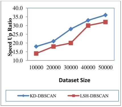
[image:6.595.52.269.282.656.2]Figures 6 and 7 show the effect of varying dataset size on clustering efficiency and speed of clustering while using synthetic dataset. The speed efficiency was calculated as the ratio of time taken by DBSCAN algorithm to the time taken by the proposed KD/LSH algorithm.
Figure 6 : Dataset Size and Clustering Efficiency
Figure 7 : Dataset Size and Time Efficiency
Careful scrutiny of the silhouette measure results show that the proposed algorithms are efficient in terms of scalability. This is evident from the increased silhouette width obtained by both KD-DBSCAN and LSH-DBSCAN algorithms. The performance of the traditional DBSCAN algorithm goes down for large-sized datasets. Thus, the speed optimizes KD-Tree and LSH have encouraging results with
respect to clustering efficiency. From figures 6 and 7, it is clear that the time efficiency gained by the proposed algorithm is high. The speed up ration obtained by KD-DBSCAN was in the range 18-33, while it was in the range 1-32 for LSH-DBSCAN. This shows that the KD-DBSCAN algorithm is more efficient than LSH-DBSCAN.
5.CONCLUSION
In this paper, the disadvantage that the traditional DBSCAN algorithm cannot handle large datasets in an efficient manner is solved by two algorithms. The first is the use of KD-Tree instead of the R-Tree algorithm used in traditional DBSCAN.
The second method included a Locally Sensitive Hashing algorithm to speed up the neighborhood search process. Both the algorithms were further enhanced by using an automated method using a k-distance graph method for calculating the input parameters, Eps and MinPts, of traditional DBSCAN. Experimental results proved that while both the algorithms improved the efficiency of DBSCAN with respect to clustering efficiency and speed, the KD-Tree based DBSCAN produced the best results. The main advantages of both the approaches are that they are unsupervised methods (which means new data can be added to the database can be clustered in future in an efficient manner) and are fully automatic and require no input from the users. Thus, the proposed algorithms are suitable for clustering both small and large sized datasets. Future work includes further research to find out reasons for the small degradation shown by LSH algorithm. Plans are also made to include pruning techniques and change of Hamming distance measure to a more efficient measure with which further speed gain can be achieved.
REFERENCES
[1] Bayer, U., Comparetti, P.M., Hlauschek, C., Kruegel, C. and Kirda, E. (2009) Scalable, behavior-based malware clustering, Proceedings of the 16th Annual Network and Distributed System Security Symposium (NDSS 2009), Pp. 1-18.
[2] Bentley, J.L. (1975) Multidimensional binary search trees used for associative searching, Communications of the ACM, Vol.18, No.9, Pp.509-517.
[3] Bhakare, K.R., Krishna, R.K. and Bhakare, S. (2012) An Energy-Efficient Grid based Clustering Topology for a Wireless Sensor Network, International Journal of Computer Applications, Vol. 39, No.14, Pp.24-28.
[4] Borah, B. and Bhattacharyya, D. (2004) An improved sampling-based DBSCAN for large spatial databases, Proceedings of International Conference on Intelligent Sensing and Information Processing, Pp. 92–96.
[5] Cao, Y., Jiang, T. and Girke, T. (2010) Accelerated similarity searching and clustering of large compound sets by geometric embedding and locality sensitive hashing. Bioinformatics, Vol. 26, No. 7, Pp. 953-959.
[6] El-Sonbaty, Y., Ismail, M. and Farouk, M. (2004) An efficient density based clustering algorithm for large
10.0 15.0 20.0 25.0 30.0 35.0 40.0
10000 20000 30000 40000 50000
Sp
ee
d Up
Ra
tio
KD-DBSCAN LSH-DBSCAN
Dataset Size
0.5 0.6 0.7 0.8 0.9
10000 20000 30000 40000 50000
Sil
ho
uet
te
Width
[image:6.595.54.269.283.470.2]databases, 16th IEEE International Conference on Tools with Artificial Intelligence, ICTAI, Pp. 673–677.
[7] Ester, M., Kriegel, H., Sander, J. and Xu, X. (1996) A density-based algorithm for discovering clusters in large spatial databases with noise, Proc. KDD 96, Pp. 226– 231.
[8] Fan, Y. and Yuta, R. (2011) A Density-based Path Clustering Algorithm, International Conference on
Intelligent Computation and Bio-Medical
Instrumentation (ICBMI), Hubei, Pp. 224-227.
[9] Folino, G., Forestiero, A., Spezzano, G., 2009. An adaptive flocking algorithm for performing approximate clustering. Inform. Sci. 179 (18), 3059–3078.
[10]Garai, G. and Chaudhuri, B.B. (2004) A novel genetic algorithm for automatic clustering, Pattern Recognition Letters, Vol. 25, No.2, Pp. 173–187.
[11]Guo, Y., Grossman, R., Xu, X., Jäger, J. and Kriegel, H. (2002) A fast parallel clustering algorithm for large spatial databases, High Performance Data Mining, Springer, US, Pp. 263–290.
[12]http://archive.ics.uci.edu/ml/datasets.html
[13]Ivancsy, R. and Kovacs, F. (2006) Clustering techniques utilized in web usage mining, Proceedings of the 5th WSEAS International Conference on Artificial Intelligence, World Scientific and Engineering Academy and Society (WSEAS), Knowledge Engineering and Data Bases, Pp. 237-242.
[14]Jain, A.K., Mutry, M.N. and Flynn, P.J. (1999) Data Clustering: A Review, ACM Computing Surveys, Vol. 31, No. 3, Pp. 264-323.
[15]Jiang, S. and Li, X. (2009) A hybrid clustering algorithm, Fourth International Conference on Fuzzy Systems and
Knowledge Discovery, Vol. 1. IEEE Computer Society, Los Alamitos, CA, USA, Pp. 366–370.
[16]Li, J., Yi, S., Wang, X., Hu, X. and Jiang, H. (2011) A new hybrid method based on partitioning-based DBSCAN and ant clustering, Expert Systems with Applications, Elsevier, Vol. 38, Issue 8, Pp.9373-9381.
[17]Phung, D., Adams, B., Tran, K., Venkatesh, S. and Kumar, M. (2009) High Accuracy Context Recovery using Clustering Mechanisms, In proceedings of the seventh international conference on Pervasive Computing and Communications, PerCom Galveston, USA, Pp. 122-130.
[18]Raiser, S., Lughofer, E., Eitzinger, C. and Smith, J.E. (2010) Impact of object extraction methods on classification performance in surface inspection systems, Special Issue Paper, Machine Vision and Applications, Springer-Verlag, PP. 627~641.
[19]Sakellariou, R., Gurd, J., Freeman, L., Keane, J., Arlia, D. and Coppola, M. (2001) Experiments in parallel clustering with DBSCAN, Euro-Par 2001 Parallel Processing, CASES’04, Springer, Berlin/Heidelberg, Vol. 2150, Pp. 26–331.
[20]Tsai, C. and Sung, C. (2010) EIDBSCAN: An extended improving DBSCAN algorithm with sampling techniques. International Journal of Business Intelligence and Data Mining, Vol. 5, No. 1, Pp.94–111.