Suitable Node Deployment based on Geometric Patterns Considering Fault Tolerance in Wireless Sensor Networks

Suitable Node Deployment based on Geometric

Patterns Considering Fault Tolerance in Wireless

Sensor Networks

Mahdie Firoozbahrami

Department of Computer Engineering, Science and Research Campus, Islamic Azad

University Hamedan, Iran

Amir Masoud Rahmani

Department of Computer Engineering, Science and Research Campus, Islamic Azad

University Tehran, Iran

ABSTRACT

Wireless Sensor Networks (WSNs) consist of small power-constrained nodes with sensing, computation and wireless communication capabilities. These nodes are deployed in the sensing region to monitor especial events such as temperature, pollution, etc. They transmit their sensed data to the sink in a multi-hop manner. The sink is the interface between sensor nodes and the end-user. It is responsible for integrating the received data from sensors and delivered the requested data to the user. Node deployment is an important issue in WSNs and can be random or deterministic. A proper node placement can increase connectivity, coverage and lifetime of a WSN. In this paper a novel deployment is proposed in which nodes are placed on two Archimedean spirals that are nested (Nested Spirals). This pattern is five-coverage and five-connected. Analytical results show that our proposed pattern uses fewer nodes than other models such as triangle, square and hexagon. Simulation results also show that our model consumes less energy than other models, so its lifetime and fault tolerance is also higher than regular patterns.

Keywords

Node Deployment, Placement, Spiral, Coverage, Connectivity, Energy Consumption, Lifetime, Wireless Sensor Network

1.

INTRODUCTION

A WSN is composed of a large number of sensor nodes that work with battery [1]. They are deployed in a region of interest for the purpose of monitoring physical or environmental conditions such as temperature, sound, vibration, pressure, motion or pollutants. They sense particular events and report them to a remote base station or sink [2]. WSNs have lots of applications [3, 4] which mainly classified into two categories: monitoring and tracking. Examples of monitoring applications are health and wellness monitoring, power monitoring, factory and process automation monitoring. Tracking objects, animals, humans and vehicles are examples of tracking applications [1]. Node deployment is an important factor in WSNs [5] and can be random or deterministic [6]. In random deployments,

sensors may be scattered by aircraft [7]. In this way sensors may not be placed in exactly their desired locations because of wind or buildings, so the coverage and connectivity of the network may be less than the requirements of the application. To avoid these problems, it is preferred to use deterministic deployment in physically accessible places. In deterministic deployments the place of nodes is known prior to deployment. If nodes deploy in a good pattern, it can reduce cost, energy consumption and increase coverage, connectivity, lifetime and fault tolerance of a WSN [8]. However finding optimal patterns for WSNs is a hard problem [9].

The rest of this paper is as follows. In section 2 some related works are discussed. Section 3 gives the details of spiral deployment. Section 4 presents our work and the way of finding number of required nodes and coordination of them. The performance study is presented in section 5. Finally conclusions and suggestions for future work are drawn in section 6.

2.

RELATED WORKS

square, hexagon and triangle patterns which are shown in figure 1. They also presented the formula to calculate number of required nodes according to their sensing radius (a) and the desired area in these three models.

(a) (b) (c)

Fig 1: (a) Square, (b) Hexagon, (c) Triangle deployment [12]

Triangle-Hexagon Tiling (THT) was also proposed in [13] and was compared with random and square grid patterns in case of coverage, energy consumption and worst-case delay. Figure 2 shows these three deployments.

It was considered that the desired sensing region is circular. THT pattern outperforms than two other strategies for energy consumption and worst-case delay. For coverage performance, a square grid is better than other strategies. Our work aims to develop a deterministic node deployment with higher coverage, greater connectivity with fewer nodes than regular patterns discussed in [12].

3.

ROBLEM STATEMENTS

Several node deployments have been proposed [12, 13]. In this paper a new pattern for node deployment is proposed with considering following assumptions:

1- The wireless sensor network is homogeneous. 2- The area is two-dimensional.

3- The communication and sensing radius of all sensors are the same.

The problem is how to deploy fewer sensors in the area (A) to achieve higher coverage and connectivity than other deployments such as square, hexagon and triangle. Before explaining our model some definitions are presented here. Definition 1:

K-Coverage: A WSN is called K-Coverage if every point of the specified area is covered by at least k sensors [13].

Definition 2:

K-Connected: A WSN is K-Connected if k-1 nodes fail and the network remains connected [8].

Definition 3: Fault Tolerance:

If the network continues to work properly in spite of failure, it is a fault tolerant network [6].

3.1

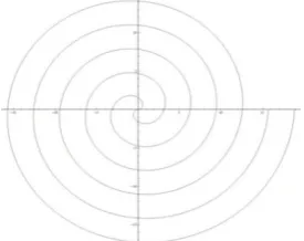
Archimedean Spiral

Its polar coordination is that “a” determines the start of turning and “b” shows the distance of consequent turnings. One feature of Archimedean spiral is that the distance of consequent turnings are the same and is equal to 2πb [14, 15, 16].

Fig 3: Archimedean spiral with polar coordination

The figure 3 shows that if nodes deploy in this mode, the WSN will be one-connected and failure of one node cause the network to be disconnected. For this reason it was decided to use two Archimedean spirals in a way to guarantee five-coverage and five-connectivity.

3.2

Nested Spirals

The proposed model is composed of two spirals with polar coordinates of and . Nested spirals with polar coordinates of (0< ) and (0< ) are shown in figure 4. The turning of spiral with polar coordination of is one less than spiral with polar coordination of . This will be useful in calculating number of nodes.

(a) (b) (c)

Fig 4: Nested spirals with polar coordinates of (0< ) and (0< )

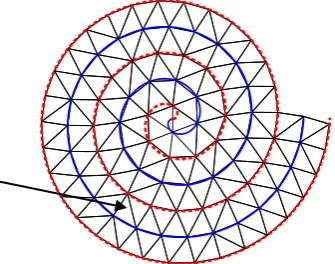
The coverage and connectivity of nested spirals are shown in figures 5 and 6. The figures show that minimum connectivity and coverage of nested spirals is five, it means that our proposed model is five-connected and five-coverage.

Fig 5: Coverage of nested spirals pattern

Fig 6: Connectivity of nested spirals pattern

4.

PROPOSED APPROACH

In this paper a new deployment of sensors is proposed in which nodes are placed on two Archimedean spirals. It is considered that the network is homogenous and the area is two dimensional. The goal is to gain higher coverage and greater connectivity by using fewer nodes. The result of our proposed deployment is a five-coverage and five-connected network. In order to compare our model with other deployments, a formula is required to get the number of nodes according to sensing/communication radius and the area. To reach the formula following steps should be determined.

1- Node’s distance in each spiral based on sensing radius.

2- Polar equation of spirals based on sensing radius. 3- Perimeter based on sensing radius and area.

By dividing the perimeter to node’s distance the number of required nodes is determined.

4.1

Node’s Distance in Each Spiral

Based on Sensing Radius

In figure 7, two spirals are shown which one of them is specified by thick blue line and the other with dashed red line.

The part which is shown by a trigger is the maximum distance that two sensors may have from each other and it is equivalent to communication radius (a). So the distance of sensors in each spiral is calculated as below:

Fig 7: Maximum distance of two sensors in nested spirals pattern

(1)

And

(2)

It means that if there are sensors with communication radius of “a”, the sensor nodes are placed in distance of from each other in each spirals.

4.2 Polar Equation of Spirals Based

on Sensing Radius

In each spirals the distance between two consecutive turnings is twice the node’s distance (d) [14]. So

(3)

By substituting “d” from equation 2, “b” will be as follows:

(4)

And the polar coordination of two nested spirals will be

π

π

(5)

π

(6)

4.3

Perimeter Based on Sensing

Radius and Area

The perimeter of Archimedean spiral with polar equation of

is calculated as follows [17]:

As explained before the turning of Archimedean spiral with polar equation is one less than spiral with polar equation of , so the perimeter of it is calculated as follows:

π (8)

Our goal is to express the perimeter based on sensing range (a) and area (A), so the area of Archimedean spiral with polar equation is presented below [18]:

A= π = π (9)

π (10)

So by substituting and

π π in equations 7 and 8

perimeters of two spirals will be

(11)

(12)

After substituting “b” according to equation 4 the perimeters will be as follows

π π π π

(13)

π π π π

π π

(14)

4.4 Formula to Calculate Number of

Required Nodes Based on Area and Sensing

Radius

Now it is enough to divide perimeters to the distance of deployed nodes (d) according to equation 2 to calculate the number of nodes in each spiral which are shown by and respectively:

π π π π

π

(15)

_π

π π π

π

π π

And the total number of nodes (N) which are required in our model is the sum of nodes in two spirals:

₍₁₇₎

4.5 Coordination of Node Placement

As explained before our model is a deterministic model in which the place of nodes is determined before deployment. For calculating the coordination of nodes in each spiral a starting point is considered and the coordination of a point with distance of “d” from that starting point is calculated and the next place will be calculated from this point and this will be repeated to get the coordination of all sensor nodes.

5. PERFORMANCE EVALUATION

In this section our proposed model is compared from different points of view with other models.

5.1 Performance Evaluation:

Coverage and Connectivity

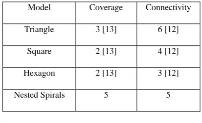
Amount of Coverage and degree of connectivity related to different models is presented in table1 [12,13]. Coverage and connectivity of different deployments is affected respectively by sense and communication radius [2]. According to section 3 and figures 5 and 6, it is concluded that our proposed model is five-coverage and five-connected. Five-coverage means that every point of the specified area is covered by at least five sensor nodes and five-connectivity means that if four neighbor sensor nodes fail, the network remains connected.

Table 1: Coverage and connectivity related to different models

Model Coverage Connectivity

Triangle 3 [13] 6 [12]

Square 2 [13] 4 [12]

Hexagon 2 [13] 3 [12]

Nested Spirals 5 5

5.2 Performance Evaluation: Number

of Required Nodes

The formula for calculating the number of nodes in our model explained in section 3.4. In order to find the number of required nodes (N) in a specified area (A) according to sensing radius in other three models, the area (A) should be divided to the average number of required nodes for every pattern. For example in square model every vertex of a square is connected to four other vertexes, so in average every square needs one node, so by calculating the area to the area of one square with length ( ), the number of required nodes will be calculated. In Triangle every vertex is connected to six other vertexes, so one triangle needs nodes in average, so after dividing the area to the area of one triangle with length and finding the number of required triangles in a specified area, it should be multiplied in . In Hexagon every vertex is connected to three other nodes, so nodes are required for every hexagon in average. After calculating the number of hexagons by dividing the specified area to the area of one hexagon, it should be multiplied in [12]. The results of calculation are presented in Table 2.

Table 2: Formulas for calculating number of nodes based on area and sensing radius

Number of nodes Model

N=1.15 [12] Triangle

N= [12] Square

N=0.77 [12] Hexagon

In this section the number of required nodes of different models is calculated for different areas and sensing ranges of 10, 20 and 30 meters. The results are presented in table 3-5.

Table 3: Number of nodes in different areas with sensing radius of 10 meters in different models

Area(m2) Model

103 104 105 106 107 108

Triangle 12 115 1150 11500 115000 1150000 Square 10 100 1000 10000 100000 1000000

hexagon 8 77 777 7777 77777 777777 Nested

spirals 28 146 722 3465 16335 76373

Table 4: Number of nodes in different areas with sensing radius of 20 meters in different models

Area(m2) Model

103 104 105 106 107 108

Triangle 3 29 287 2875 28750 287500

Square 3 25 250 2500 25000 250000

hexagon 2 20 192 1925 19250 192500

Nested

spirals 10 54 277 1352 6431 30193

Table 5: Number of nodes in different areas with sensing radius of 30 meters in different models

Area(m2) Model

103 104 105 106 107 108

Triangle 2 13 127 1277 12777 127777

Square 2 12 111 1111 11111 111111

hexagon 1 9 85 855 8555 85555

Nested

spirals 6 30 157 776 3719 17530

5.2.1 Improvement Point

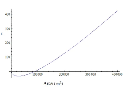
If the formula to calculate the number of nodes based on area and sensing radius in other models such as triangle and nested spiral are shown respectively by F1 and F2, F is expressed as follows:

F= F1- F2

If the value of F is positive, It means that F1 is higher than F2 , so triangle model requires more nodes than nested spirals and if its value is negative, It can be concluded that our model needs fewer nodes than triangle model.

The plot of F for different areas and sensing radius is shown in figures 8-10. Results show that nested spirals needs fewer nodes than triangle model from areas of 22000, 90000 and 200000 respectively with radius sense of 10, 20 and 30 meters. The same calculation can be done for hexagon and square patterns to determine the improvement point of nested spiral.

Fig 8: Value of F with different area(A) and sensing radius 10 meters

Fig 9: Value of F with different area(A) and sensing radius

20 meters

Fig 10: Value of F with different area(A) and sensing radius 30 meters

5.3 Performance Evaluation: Energy

Consumption

In order to compare energy consumption of models with each other, they are simulated with ns2 with the parameters which are listed in table 6.

Table 6: WSN’s Simulation parameters

Standard of MAC 802.15.4

Routing Protocol AODV

Initial Energy of each sensor 50 J Energy consumption for sending and

receiving per second

0.02 J

Sensing /Communication radius 10 meters

Packet size 60 bytes

Number of Packets sent per second 20 packets

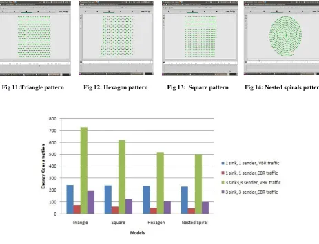
Figure 15 and 16 shows that our proposed model uses less energy than other three models. The reason is that in other models the distances of nodes is exactly the same as

communication radius but in our model nodes are placed in distances less than communication radius, so they consume

Fig 11:Triangle pattern Fig 12: Hexagon pattern Fig 13: Square pattern Fig 14: Nested spirals pattern

Fig 15: Energy consumption in different scenarios with 100 nodes

Fig 16: Energy consumption in different scenarios with 400 nodes

0 200 400 600 800 1000 1200

Triangle Square Hexagon Nested Spiral

En

er

g

y

Co

n

sum

p

ti

o

n

Models

less energy for sending and receiving packets. Less energy consumption cause higher lifetime and greater fault tolerance.

6. CONCLUSION AND FUTUER

WORK

In this paper a new deployment pattern for WSNs is proposed and analyzed. In our model, sensor nodes are placed in a spiral pattern in distances less than communication radius to guarantee five-coverage and five-connectivity. Our proposed model has higher coverage than other models such as triangle, square and hexagon. Its connectivity is also greater than square and hexagon deployments. Analytical results show that our model uses fewer sensors than other models when the ratio of area to sensing radius is high. Simulation results show that the proposed model consumes less energy than other models, so the lifetime and fault tolerance of our model is greater than other models.

Here a new deployment pattern is proposed, it is suggested to schedule sensor nodes in a way that reduced set of sensors remain active in the execution of a sensing task to increase network lifetime [19]. Also in this paper homogenous wireless sensor network is considered, so it is suggested to use spiral deployment in heterogonous wireless sensor network and using other kinds of spirals such as logarithmic ones.

REFERENCES

[1] J. Yick, B. Mukherjee, D. Ghosal, ‘‘Wireless sensor network survey”, Computer Networks 52, pp. 2292-2330, 2008.

[2] Y. Ch. Wang, ‘‘Efficient deployment algorithms for ensuring coverage and connectivity of wireless sensor networks”, Proceedings of the First International Conference on Wireless Internet, pp. 114-121, July 2005. [3] I. F. Akyildiz, W. Su, Y. Sankarasubramaniam, E. Cayirci, ‘‘Wireless sensor networks: a survey”, Computer Networks, Vol.38, no. 4, pp. 393-422, 2002. [4] J. Burrell, T. Brooke, and R. Beckwith. Vineyard

computing: sensor networks in agricultural production. IEEE Pervasive Computing, Vol. 3, no. 1, pp.38-45, 2004.

[5] C. Y. Chang, J. P. Sheu, ‘‘An obstacle-free and power-efficient deployment algorithm for wireless sensor networks”, IEEE transactions on systems, man, and cybernetics-part A: systems and humans, vol. 39, no. 4, July 2009.

[6] A. Zheng, J. Jamalipour, ‘‘WIRELESS SENSOR NETWORKS A Networking Perspective”, New Jersey: John Wiley & Sons, 2009.

[7] P.Gajbhiye, A. Mahajan, ‘‘a survey of architecture and node deployment in wireless sensor network”, First International Conference on Applications of Digital Information and Web Technologies (ICADIWT), pp. 426-430, Aug. 2008.

[8] J. L. Bredin, E. D. Demaine, M. T. Hajiaghayi, D. Rus, ‘‘Deploying sensor network with guaranteed fault tolerance”, Journal of IEEE/ACM Transactions on Networking (TON), Vol.18, pp. 216-228, 2010.

[9] X. Bai, Z. Yun, D. Xuan, T. H.Lai, W. Jia, ‘‘Deploying four-connectivity and full-coverage wireless sensor networks”,27th Conference on Computer Communication (INFOCOM), pp. 296-300, April 2008. [10] S.Meguerdichian, F. Koushanfar, M. Potkonjak, and M.

B. Srivastava, ‘‘Coverage problems in wireless ad-hoc sensor networks”, In INFOCOM, pp. 1380-1387, 2001. [11] H. Zhang and J. C. Hou, ‘‘ Maintaining sensing coverage

and connectivity in large sensor networks”, In NSF International Workshop on Theoretical and Algorithmic Aspects of Sensor, Ad Hoc Wireless and Peer-to-Peer Networks, 2004.

[12] E .S. Biagioni, G .Sasaki , ‘‘Wireless sensor placement for reliable and efficient data collection”, Proceedings of the 36th Annual Hawaii International Conference on System Sciences, Jan. 2003.

[13] W. Y. Poe, J. B. Schmitt, ‘‘Node deployment in large wireless sensor networks: coverage, energy consumption, and worst-case delay”, Proceedings of Asian Internet Engineering Conference, pp. 77-84, 2009.

[14] http://en.wikipedia.org/wiki/Archimedeanspiral [15] http://mathworld.wolframe.com/ArchimedesSpiral.html [16] http://www.mathematische-basteleien.de/spiral.htm [17] http://fiji.sc/downloads/snapshots/arc_length.pdf [18] R. Smith, R. Minton, ‘‘Calculus: Early Transcendental

Functions”, 4th edition, United States: McGraw-Hill, 2012

[19] M. Mappar, A. M. Rahmani, A. H. Ashtari, “A new approach for sensor scheduling in wireless sensor networks using simulated annealing”, 4th