Complex and Inverse Complex Dynamics of Fractals using Ishikawa Iteration

(1)

Complex and Inverse Complex Dynamics of Fractals

using Ishikawa Iteration

Ashish Negi

Associate Professor Dept. of Computer science and

Engineering

G.B.Pant Engineering College Ghurdauri, Pauri

Shashank Lingwal

Dept. of Computer Science and Engineering

Yashwant Singh Chauhan

Astt. Professor

Dept. of Computer Science and Engineering

ABSTRACT

Complex graphics of dynamical system have been a subject of intense research nowadays. The fractal geometry is the base of these beautiful graphical images. Many researchers and authors have worked to study the complex nature of the two most popular sets in fractal geometry, the Julia set and the Mandelbrot set, and proposed their work in various forms using existing tools and techniques. Still researches are being conducted to study and reveal the new concepts unexplored in the complexities of these two most popular sets of fractal geometry. Recently, Ashish Negi, Rajeshri Rana and Yashwant S. Chauhan are among those researchers who have contributed a lot in the area of Fractal Geometry applications. In this paper we review the recently done work on complex and inverse complex functions for producing beautiful fractal graphics. The reviewed work mainly emphasizes on the study of the nature of complex and inverse complex functional dynamics using Ishikawa iterates and existence of relative superior Mandel-bar set.

Keywords

Fractals, Complex dynamics, Inverse Complex dynamics, Relative Superior Mandelbrot Set, Relative Superior Julia Set, Ishikawa Iteration, Relative Superior Mandel-bar Set.

1. INTRODUCTION

In 1918, French mathematician Gaston Julia [9] investigated the iteration process of complex function and attained a Julia set, which is a landmark in the field of fractal theory. The object Mandelbrot set on the other hand was given by Benoit B. Mandelbrot [11] in 1979. The visual complexity, beauty and self similarity of these structures have made these subjects of a wide area of intense research right from its advent. The various extensions and variants of both of these sets have been extensively studied using Picard’s iterations. We have applied in this research article a new iteration process called Ishikawa iteration.

The fractals generated from the self-squared function

z



z

2



c

, where z and c are complex quantities, have been studied extensively in literature [5, 6, 7 & 14]. Recently, the generalized transformation function

n

z



z





c

for positive integer value of n has been considered by K.W.Shirriff [14]. The z plane fractal images for the function

z

_n_₁



z

_n



c

for positive and negative, both integer and non-integer values of n have been presented

by Gujar et al. along with some conjectures about their visual characteristics [6, 7].

Several programs and papers have used escape-time methods to produce images of fractals based on the complex mapping

1

( n )

z z c  , where exponent n is a positive integer. On the other hand, Shizuo [15], has presented the various properties of Multicorns and Tricorns for simple complex function, where z and c are complex quantities. Shizuo[16]has also quoted the Multicorns as the generalized Tricorn or Tricorn of higher order. The dynamics of anti-polynomial

d

zz c of complex polynomial d

z c, where

2 d



, leads to interesting Tricorns and Multicorns antifractals with respect to function iteration[4, 15, 16]. Multicorns are symmetrical objects. Their symmetry has been studied by Lau and Schieicher [10]. The study of connectedness locus for anti-holomorphic polynomials

2

z c defined as Tricorns coined by Milnor, plays an intermediate role between quadratic and cubic polynomials. Crowe etal.[3] considered as in formal analogy with Mandelbrot set and named it as Mandel-bar set and also brought its features bifurcations along axis rather than at points. Milnor [12] found it as a real slice of cubic connected locus. Winters [17] showed it as boundary along the smooth arc.

In this paper we considered the transformation (for studying complex dynamics) of the functions

z



z

2



c

_,

n



2

and

z



z

n



c

_,

n



2

, and transformation (for studying inverse complex dynamics) of the function

1

( n )

z z c  , for

n



2

, and analysed the z plane fractal images for the first function and c plane fractal images for the second function, generated from Ishikawa iterations of these functions using Ishikawa iteration procedure. We explored the drastic changes that occur in visual characteristics of the images for different integer and non-integer values of n.

2. ELABORATION OF CONCEPTS

INVOLVED

2.1 Mandelbrot Set

Definition 1. The Mandelbrot set M for the quadratic 2

( ) = z + c

C

(2)

c



C

for which the orbit of point 0 is bounded, that is, { :{ n(0)}; 0,1, 2, 3... is bounded}

c

M  cC Q n

An equivalent formulation is

{ :{ n(0) does not tends to as }} c

M  cC Q  n 

We choose the initial point 0, as 0 is the only critical point of Qc .

2.2 Julia Set

Definition 2. The set of points K whose orbits are bounded under the iteration function of Qc(z) is called the Julia set. We

choose the initial point 0, as 0 is the only critical point of Qc(z) .

2.3 Ishikawa Iteration

Definition 3. Ishikawa Iterates[8]: Let X be a subset of real or complex number and f :X X for all x₀X, we

have the sequence {xn} and {yn} in X in the following

manner:

' ( ) (1 ' )

n n n n n

y S f x  S x

1 ( ) (1 )

n n n n n

x S f y  S x

where 0S'_n 1, 0S_n 1 and S'_n & S_n are both convergent to non-zero number.

2.4 Relative Superior Orbit

Definition 4. [13] The sequence xn and yn constructed above

is called Ishikawa sequence of iteration or relative superior sequence of iterates. We denote it by

0

( , n, ' , )n

RSO x s s t .

Notice that

0

( , _n, ' , )_n

RSO x s s t with s'_n 1 is

0

(

,

_n

, )

SO x s t

i.e. mann’s orbit and if we place

' 1

n n

s s  then

0

( , _n, ' , )_n

RSO x s s t reduce to

0

(

, )

O x t

. We remark that Ishikawa orbit

0

( , n, ' , )n

RSO x s s t with s'n 1 / 2 is relative superior

orbit.

2.5 Relative Superior Mandelbrot Set

Now we define Mandelbrot set for the function with respect to Ishikawa iterates. We call them as Relative Superior Mandelbrot sets.

Definition 5. [13] Relative Superior Mandelbrot set RSM for the function of the form _{( )} n

c

Q z z c, where n = 1,2,3,… is defined as the collection of

c



C

for which the

orbit of 0 is bounded i.e.

{ : ck(0) : 0,1, 2, 3...}

RSM  cC Q k is bounded.

In functional dynamics, we have existence of two different types of points. Points that leave the interval after a finite number are in stable set of infinity. Points that never leave the interval after any number of iterations have bounded orbits.

2.6 Relative Superior Julia Set

Definition 6. [2] The set of points RSK whose orbits are bounded under relative superior iteration of function Q(z) is called Relative Superior Julia sets. Relative Superior Julia set of Q is boundary of Julia set RSK.

2.7 Mandel-bar Set

Definition 7. [2] The Mandel-bar set Ac , for the quadratic

( ) 'n c

A z z c is defined as the collection of all cC for which the orbit of point 0 is bounded, that is,

0,1,2,3,...

{ : (0) is bounded}

c c n

A  cC A  .

An equivalent formulation is

{ : (0) not tends to as n }

c c

A  cC A    .

2.8 Relative Superior Mandel-bar Set

Definition 8. [13] Relative superior Mandel-bar set RSMB for the function of the form _{( )} n

c

Q z z c, where n=1,2,3,4,… is defined as the collection of cC for which

the orbit of 0 is bounded i.e.

{ : k(0) : 0,1, 2, 3,...} c

RSMB cC Q k is bounded.

3. GENERATING PROCESS

The basic principle of generating fractals employs the iterative formula:

1 ( )

n n

z _  f z where z0 = the initial valueof z,

and zi = the value of complex quantity z at the ith iteration [6,

7]. For example, the Mandelbrot’s self-squared function for generating fractal is: f(z) = z2+c , where z and c are both complex quantities. We propose the use of transformation function zznc n, 2 and 1

( n )

z z c  for generating fractal images with respect to Ishikawa iterates, where z and c are the complex quantities and n is a real number. Each of these fractal images is constructed as two-dimensional array of pixel. Each pixel is represented by a pair of (x,y) coordinates. The complex quantities z and c can be represented as:

x y

zz iz

x y

cc ic

where _i_ _{( 1)}_ and zx , cx are the real parts and zy , cy are

the imaginary parts of z and c respectively. The pixel coordinates (x,y) may be associated with (cx,cy) or (zx,zy) .

Based on this concept, the fractal images can be classified as follows:

(a) z-Plane fractals, wherein (x,y) is a function of (zx,zy).

(b) c-Plane fractals, wherein (x,y) is a function of (cx,cy).

(3)

4. ESCAPE CRITERION FOR

RELATIVE SUPERIOR JULIA AND

MANDELBROT SETS

4.1 Escape Criterion for Quadratics

[13] Suppose that z max{c, 2 / , 2 / '}s s , then

(1 )n n

z   z and z   as

n

 

. So, z  c and z 2 /s as well as z 2 /s' shows the escape criteria for quadratics.

4.2 Escape Criterion for Cubics

[13] Suppose 1/ 2 1/ 2

max{ , ( 2 / ) , ( 2 / ') }

z  b a  s a  s

then

n

z   as

n

 

. This gives the escape criterion for cubic polynomials.

4.3 General Escape Criterion

[13] Consider _z _max{_c_{, (2 / )}_s 1/ 2_{, (2 / ')}_s 1/ 2_}_then

n

z   as

n

 

is the escape criterion.

Note that the initial value z0 should be infinity, since infinity

is the critical point of 1

( n )

z z c  . However, instead of starting with z0 = infinity, it is simpler to start with z1 = c,

which yields the same result. A critical point of ( )

zF z c is a point whereF'( )z 0.

5. SIMULATIONS AND RESULTS

Generation of Relative Superior Mandelbrot set

Fig.1: For cubic function [1]: s=0.8, s’=0.3, n=3.2

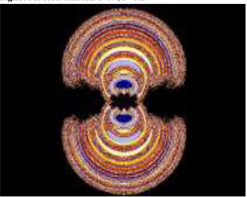
Fig.2: For cubic function: s=0.8, s’=0.3, n=3.8

Fig.3: For bi-quadratic function: s=0.5, s’=0.4, n=4.2

Fig.4: For bi-quadratic function: s=0.5, s’=0.4, n=4.8

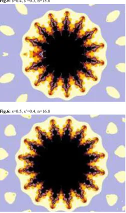
[image:3.595.314.568.81.281.2] [image:3.595.315.565.301.502.2] [image:3.595.54.305.453.651.2] [image:3.595.315.557.524.718.2]

(4)

Fig.5: s=0.4, s’=0.3, n=15.8

Fig.6: s=0.5, s’=0.4, n=16.8

Generation of Relative Superior Julia Sets:

(for cubic function)

Fig.7: s=0.5, s’=0.4, n=3.2 c=0.03488180321-0.01680604855i

Fig.8: s=0.5, s’=0.4, n=3.8 c=-0.0442117701+0.03592300032i

(for bi-quadratic function)

Fig.9: s=0.8, s’=0.2, n=4.2 c=0.04015470789+0.03592299963i

[image:4.595.55.308.76.503.2] [image:4.595.57.577.82.769.2] [image:4.595.317.567.95.292.2]

(5)

Generalization of Relative Superior Julia Sets:

Fig.11: s=0.5, s’=0.4, n=15.8

c=-0.001391094496+0.005718433219i

Fig.12: s=0.5, s’=0.4, n=16.8 c=-0.06389131715+0.02134348888i

Fixed points :

[image:5.595.116.554.98.731.2]

Fixed points of Quadratic Polynomial [13] :

Table 1: Orbit of F(z) at s=0.5 and s’=0.1 for (z0=-0.01192288639+0.01042379668i)

Number of

iteration i |F(z)|

Number of

1 0.015837 6 0.85943

2 0.98458 7 0.85943

3 0.86429 8 0.85942

4 0.85883 9 0.85942

5 0.85933 10 0.85942

Fig.13: Observation : the value converges to a fixed point after 08 iterations

[image:5.595.317.564.108.304.2]

Fixed points of Cubic polynomial [13]

Table 2 : Orbit of F(z) at s=0.5 and s’=0.1 for (z0=-0.00888346751+0.01650347336i)

Number of

1 0.018742 6 0.86749

2 0.97928 7 0.86747

3 0.85738 8 0.86747

4 0.86871 9 0.86747

5 0.86732 10 0.86747

[image:5.595.52.304.116.314.2] [image:5.595.316.565.504.709.2]

(6)

Fixed points of Bi-quadratic polynomial [13]

Number of

1 0.040014 8 0.8968

2 0.98215 9 0.89704

3 0.90556 10 0.89699

4 0.88426 11 0.89699

5 0.90308 12 0.89699

6 0.89476 13 0.89699

[image:6.595.314.567.81.281.2]

7 0.8977 14 0.89699

[image:6.595.54.303.304.504.2]

Generation of Relative Superior Mandelbrot Set:

Fig.16: For quadratic function: s=0.8, s’=0.3

Fig.17: For cubic function: s=0.8, s’=0.3

[image:6.595.314.567.333.530.2]

Generation of Relative Superior Julia Sets:

[image:6.595.54.305.541.744.2]

Fig.18: For quadratic function: s=0.5, s’=0.4 c=0.002169194079+0.465750756i

[image:6.595.313.567.566.760.2]

(7)

Fixed points :

[image:7.595.309.552.70.196.2]

Fixed points for quadratic polynomial [2]:

Number of

1 0.61619 14 0.35866

2 0.5189 15 0.35835

3 0.288 16 0.35852

4 0.43079 17 0.35842

5 0.32218 18 0.35848

6 0.37886 19 0.35845

7 0.34703 20 0.35846

8 0.36492 21 0.35845

9 0.35484 22 0.35846

10 0.36049 23 0.35846

11 0.35732 24 0.35846

12 0.3591 25 0.35846

[image:7.595.49.290.138.387.2]

13 0.3581 26 0.35846

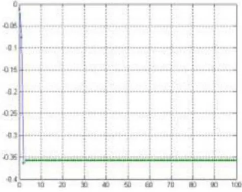
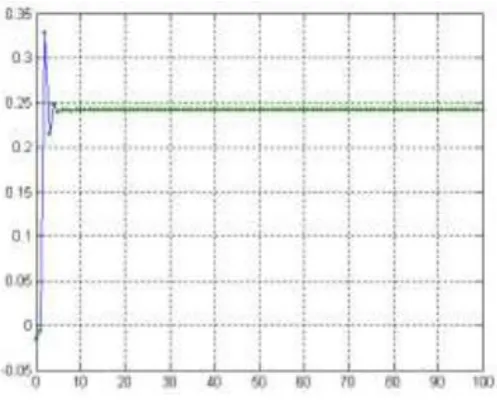
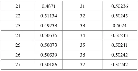
Fixed points for cubic polynomial [2]:

Table 5: Orbit of F(z) at s=0.4 and s’=0.2 for (z0=-0.0189704705+0.02867852789i)

Number of

18 0.6098 28 0.50274

19 0.45643 29 0.50223

20 0.52977 30 0.50252

21 0.4871 31 0.50236

22 0.51134 32 0.50245

23 0.49733 33 0.5024

24 0.50536 34 0.50243

25 0.50073 35 0.50241

26 0.50339 36 0.50242

[image:7.595.315.563.220.438.2]

27 0.50186 37 0.50242

Fig.21: Observation : we skipped 17 iteration and the value converges to a fixed point after 36 iterations

Generation of Relative Superior Mandel-bar Set:

[image:7.595.54.300.412.627.2] [image:7.595.314.566.468.676.2]

(8)

[image:8.595.54.306.80.281.2] [image:8.595.315.565.96.290.2]

Fig.23: For cubic function: s=0.4, s’=0.2

Fig.24: For bi-quadratic function: s=0.6, s’=0.2

Fig.25: Generalization of RSMB : s=0.5, s’=0.2, n=19

[image:8.595.54.303.296.502.2]

Generation of Relative Superior Julia Sets for Mandel-bar set:

Fig.26: For quadratic function: s=0.6, s’=0.2,

c=0.08166620257+0.00739899807i

Fig.27: For cubic function: s=0.8, s’=0.3,

c=-0.003854849909+0.01666833389i

6. CONCLUSION

 The z plane fractal image for the function 2

z



z



c

,

n



2

showed that the stable region is bounded by unstable region. Besides this, the non integer value change brought the embryonic structure in the form of lobe.

 On the other hand the c plane geometrical analysis of the function

_z



(

_z

n



_c

)

1

,

n



2

represented the planetary type structure comprising of central planet with satellites. Here non integer value change showed the embryonic self similar growth in satellite pattern.

[image:8.595.316.569.327.519.2] [image:8.595.54.304.525.717.2]

(9)

 The geometry of Relative Superior Mandelbrot set and Relative Superior Julia sets of inverse function showed their rotational as well as reflection symmetry. One of the most fascinating results is the central planet with satellite like structure obtained for biquadratic Relative Superior Julia sets.

 Further, for the odd value of n, all the Relative Superior Mandelbar sets are symmetrical objects, and for the even values of n, all the relative superior Mandelbar sets are symmetrical about x-axis. Besides this, our antifractals are different from the normal Tricorns and Multicorns as they have (n-1) wings.

7. ACKNOWLEDGMENTS

Our thanks to Dr. A.K. Swami, Principal, G.B.Pant Engineering College, Ghurdauri, for providing necessary infrastructure for the research work. We would also like to thank Mrs. Priti Dimri, Head, Department of Computer Science and Engineering, G.B.Pant Engineering College, Ghurdauri, for her unconditional and valuable support in writing this paper.

8. REFERENCES

[1] Yashwant S Chauhan, Rajeshri Rana, and Ashish Negi, “Complex Dynamics of Ishikawa Iterates for Non Integer Values”, International Journal of Computer Applications (0975-8887) Volume 9- No.2,October 2010

[2] Yashwant S. Chauhan, Rajeshri Rana, Ashish Negi, “Mandel-Bar Sets of Inverse Complex Function”, International Journal of Computer Applications (0975-8887) Volume 9- No.2, November 2010

[3] W.D.Crowe, R.Hasson, P.J.Rippon, and P.E.D. Strain-Clark, “On the structure of the Mandel-bar set”, Nonlinearity(2)(4)(1989), 541-553. MR1020441 [4] Robert L. Devaney, “A First Course in Chaotic

Dynamical System: Theory and Experiment”, Addison-Wesley, 1992. MR1202237

[5] S.Dhurandar, V.C.Bhavsar and U.G.Gujar, “Analysis of z-plane fractal images from

z



z





c

for





0

” Computers and Graphics 17,1(1993), 89-94

[6] U.G. Gujar and V.C. Bhavsar, “Fractals from

z



z





c

in complex c-Plane”, Computers and Graphics 15, 3 (1991), 441-449

[7] U.G. Gujar, V.C. Bhavsar and N. Vangala, “Fractals from

z



z





c

in complex z-Plane”, Computers and Graphics 15, 4 (1991), 45-49

[8] S. Ishikawa, “Fixed Points by a new iteration method”, Proc. Amer. Math. Soc.44 (1974), 147-150

[9] G. Julia, “Sur 1’ iteration des functions rationnelles”, J Math Pure Appli. 8 (1918), 737-747

[10] Eike Lau and Dierk Schleicher, “Symmetries of fractals revisited.”, Math. Intelligencer (18)(1)(1996), 45-51. [11] B. B. Mandelbrot, “The Fractal Geometry of Nature”,

W. H. Freeman, New York,1983.

[12] J. Milnor, “Dynamics in one complex variable; Introductory lectures”, Vieweg (1999).

[13] Rajeshri Rana, Yashwant S. Chauhan, Ashish Negi, “Inverse Complex Function Dynamics of Ishikawa Iterates”, International Journal of Computer Applications (0975-8887) Volume 9- No.1, November 2010

[14] K.W. Shirriff, “An investigation of fractals generated by n

z



z





c

”, Computers and Graphics 13, 4 (1993), 603-607

[15] N.Shizuo and Dierk Schleicher, “Non-local connectivity of the Tricorn and Multicorns”, Dynamical system and chaos (1) (Hachioji, 1994), 200-203, World Sci. Publ., River Edge, NJ, 1995 MR1479931

[16] N. Shizuo and Dierk Schleicher, “On multicorns and unicorns: I. Antiholomorphic dynamics. Hyperbolic components and real cubic polynomials”, Internat. J. Bifur. Chaos Appl. Sci. Engrg, (13)(10)(2003), 2825-2844.