A new parallel splitting augmented Lagrangian based method for a Stackelberg game

(1)

R E S E A R C H

Open Access

A new parallel splitting augmented

Lagrangian-based method for a Stackelberg

game

Xihong Yan

*

_{and Ruiping Wen}

*_{Correspondence:} [email protected]

Higher Education Key Laboratory of Engineering and Scientiﬁc Computing, Taiyuan Normal University, Taiyuan, Shanxi 030012, P.R. China

Abstract

This paper addresses a novel solution scheme for a special class of variational inequality problems which can be applied to model a Stackelberg game with one leader and three or more followers. In the scheme, the leader makes his decision ﬁrst and then the followers reveal their choices simultaneously based on the information of the leader’s strategy. Under mild conditions, we theoretically prove that the scheme can obtain an equilibrium. The proposed approach is applied to solve a simple game and a traﬃc problem. Numerical results about the performance of the new method are reported.

Keywords: Stackelberg game; variational inequality; separable structure; convergence; parallel splitting method

1 Introduction

In our work, we concentrate on typical structured variational inequality problems which are mathematically described as follows: Find a pointw∗∈such that

Qw∗Tw–w∗≥, ∀w∈,

where

w=

⎛ ⎜ ⎜ ⎜ ⎜ ⎝

x

x

.. . xm

⎞ ⎟ ⎟ ⎟ ⎟

⎠, Q(w) =

⎛ ⎜ ⎜ ⎜ ⎜ ⎝

f(x)

f(x)

.. . fm(xm)

⎞ ⎟ ⎟ ⎟ ⎟

⎠, =

(x,x, . . . ,xm)

xi∈Xi,

m

i=

Aixi=b

,

Xi⊆Rni, andfi:Xi→Rni (i= , , . . . ,m) are mappings. In the work, we assume that

Xi(i= , , . . . ,m) are nonempty, closed, and convex sets, the mappingsfi(i= , , . . . ,m) are monotone, and the solution of the problem exists. By attaching a Lagrange multiplier vectorλ∈Rl_{to the linear constraint}m

i=Aixi=b, the above problem can be converted

to the following form: Find a pointu∗∈U=m_i_=Xi×Rlsuch that

Fu∗Tu–u∗≥, ∀u∈U, (.)

(2)

where

u=

⎛ ⎜ ⎜ ⎜ ⎜ ⎜ ⎜ ⎜ ⎝

x

x

.. . xm

λ ⎞ ⎟ ⎟ ⎟ ⎟ ⎟ ⎟ ⎟ ⎠

and F(u) =

⎛ ⎜ ⎜ ⎜ ⎜ ⎜ ⎜ ⎜ ⎝

f(x) –ATλ

f(x) –ATλ

.. . fm(xm) –ATmλ

m

i=Aixi–b

⎞ ⎟ ⎟ ⎟ ⎟ ⎟ ⎟ ⎟ ⎠

. (.)

The structured system (.)-(.) can be viewed as a mathematical formulation of a one-leader-m-follower Stackelberg game whereith follower controls his decisionxi,i= , , . . . ,m. For the special case where the game has one leader and two followers, that is,m= , there is extensive literature on numerical algorithms [–]. Although the one-leader-two-follower game is helpful as a baseline model in analyzing games and their equilibrium-seeking algorithms, many application problems involve three or more fol-lowers, that is, they are formulated as the problem (.)-(.) withm≥. However, there is less work that focuses on designing algorithms for the general casem≥ compared to a considerable number of studies on the special casem= .

For the general case of the problem (.)-(.), we can directly employ the classical augmented Lagrangian method proposed by []. However, the classical augmented La-grangian method may prevent us from enjoying the separable structure of problem (.)-(.), since the subproblems obtained in the steps of the method involve coupled vari-ables. Frequently used and powerful ideas for dealing with the diﬃculty are decomposi-tion techniques. Based on the techniques, there are two most noteworthy categories of decomposition methods for the problem (.)-(.) in the literature: the alternating di-rection method and the parallel splitting augmented Lagrangian method. The alternating direction method has obtained recognition as a benchmark method to solve the problem (.)-(.), ever since it was proposed by Gabay and Mercier []. The application of the solution method has been extended in the past decade to cover a variety of areas [–]. The basic iterative scheme of the method for solving the problem (.)-(.) is as follows: When a decisionuk= (xk_,xk_, . . . ,xk_m,λk) is provided, the method getsxk_+,xk_+, . . . ,xk_m+by solving the following system:

⎧ ⎪ ⎪ ⎪ ⎪ ⎪ ⎪ ⎪ ⎪ ⎪ ⎪ ⎪ ⎨ ⎪ ⎪ ⎪ ⎪ ⎪ ⎪ ⎪ ⎪ ⎪ ⎪ ⎪ ⎩

(x_–x)T{f(x) –AT[λk–H(Ax+ m

j=Ajxkj–b)]} ≥, ∀x∈X, · · ·

(x_i–xi)T{fi(xi) –ATi[λk–H(

i–

j=Ajxkj++Aixi+mj=i+Ajxkj –b)]} ≥,

∀x_i∈Xi,

· · ·

(x_m–xm)T{fm(xm) –ATm[λk–H(

m–

j= Ajxkj++Amxm–b)]} ≥,

∀x_m∈Xm.

(.)

Then updateλby equation (.),

λk+=λk–H

_m

i=

Aixki+–b

, (.)

(3)

Note that the alternating direction method has been an attractive approach in that it successfully employs the Gauss-Seidel decomposition technique. However, in the method, each follower reveals his strategies sequentially, that is, the decisionxk+

i of the followeri is revealed only when his former followers’ strategiesxk+

 , . . . ,xki–+ are available, which is

not reasonable for the case where each follower is blind with the others’ strategies. As we mentioned, the other eﬃcient method to deal with the problem (.)-(.) is so-called the parallel splitting augmented Lagrangian method proposed by He [] based on Jacobian decomposition. Compared to the alternating direction method, the speciality of the parallel splitting augmented Lagrangian method is that it simultaneously solves the following subproblems to obtainxk_i+(i= , , . . . ,m):

x_i–xi

T

fi(xi) –ATi

λk–H j=i

Ajxkj +Aixi–b

≥,

∀x_i∈Xi,i= , , . . . ,m, (.)

which means that the followers make their choices simultaneously. However, there are few studies to address the convergence of the scheme (.)-(.), which results in improved methods where the output provided by (.) is corrected by a further correction step [– ]. All these methods are designed by adding a correction step as follows:

uk+=uk–αkd

uk–u˜k, (.)

whereαkis a stepsize,u˜k is output of (.) which is called a predictor, and –d(uk–u˜k) is a descent direction atuk_{. The schemes may be understood in the context of a game} in the following way: When the leader provides a decisionuk_{= (x}k

, . . . ,xkm,λk), all follow-ers decide their strategiesx˜k

i (i= , , . . . ,m) simultaneously by solving the corresponding subproblems in (.), respectively. Then, based on the feedbackx˜k_i (i= , , . . . ,m) from the followers, the leader improves his strategy by (.).

It is noted that in the schemes (.)-(.), the leader controls all decision variables which is not realistic since in many practical problems the leader only has power on his own deci-sion variables. Based on this identiﬁed research gap, the aim of this work is to devise a new method for the problem (.)-(.), that is, a mathematical formulation of a one-leader-m-follower Stackelberg game where the leader controlsλand theith follower controlsxi. In the correction step of our method, only the leader’s variableλis improved. Furthermore, we provide insights on the convergence of our method and a computational study of its performance.

The rest of the paper is organized as follows. Section  gives preliminaries, such as deﬁ-nitions and notations, which will be useful for our analysis and ease of exposition. Section  presents the proposed method in detail. Section  conducts an analysis on the global con-vergence of the proposed method. In Section , we apply the method to solve some prac-tical problems and report the corresponding computational results. Finally, conclusions and some future research directions are stated in Section .

2 Preliminaries

(4)

in the paper mean column vectors. For ease of exposition, we use the vector (x, . . . ,xm) to represent (xT_, . . . ,xT

m)T, whereTrepresents the transpose operator.δmax(A) denotes the largest eigenvalue of square matrixA. For any symmetric and positive deﬁnite matrixG, we denote byxG:=

√

xT_Gx_its_{G-norm. In the work, we deﬁne}

G=

⎛ ⎜ ⎜ ⎜ ⎜ ⎜ ⎜ ⎜ ⎝

αAT_HA αAT

HA

. ..

αAT mHAm

H–

⎞ ⎟ ⎟ ⎟ ⎟ ⎟ ⎟ ⎟ ⎠

(.)

such thatu–u∗_G:=Ax–Ax∗αH+· · ·+Amxm–Amx∗mαH+λ–λ∗H–.

Deﬁnition .

(a) A mappingf :Rn_→_Rn_{is described as a monotone function, if}

(x–x)T

f(x) –f(x)

≥, ∀x,x∈Rn.

(b) A mappingf :Rn_→_Rn_{is described as a strongly monotone function with} modulusμ> , if

(x–x)T

f(x) –f(x)

≥μx–x, ∀x,x∈Rn.

In the paper, there is a basic assumption that the mappingsfi(i= , , . . . ,m) are contin-uous and strongly monotone with modulusμfi, respectively.

3 Parallel method

In this section, we formally state the procedure of the new parallel splitting method for solving the problem (.)-(.) and provide some insights on the method’s properties.

Algorithm .(A new augmented Lagrangian-based parallel splitting method) S. Select an initial pointu= (x_, . . . ,x_m,λ)∈U,> ,α> , andH, and setk= .

S. Simultaneously obtain solutionsxk_i+(i= , , . . . ,m) by solving the following variational inequalities:

xi∈Xi,

x_i–xi

T

fi(xi) –ATi

λk–H j=i

Ajxkj+Aixi–b

≥,

∀x_i∈Xi, (.)

respectively. Then set

˜

λk=λk–H

_m

i=

Aixki+–b

. (.)

S. Updateλk+through equation (.),

(5)

S. If

max

i

Aixki –Aixki+,λk–λk+≤, (.)

stop. Otherwise, setk=k+ and go to S.

Remark . Now, we conduct some analysis on the proposed algorithm. From (.) and (.), we can deduce thatm_i_=Aixik+=bifλk+=λk. Then we have

j=iAjxkj+Aixki+–b=  under the condition thatAixki+=Aixki (i= , , . . . ,m). Furthermore, according to (.), there exist the following inequalities and equation:

xk_i+∈Xi,

x_i–xk_i+Tfi

xk_i+–AT_iλk+ ≥, ∀x_i∈Xi,i= , , . . . ,m, (.)

and

m

i=

Aixki+=b.

Thus, it is obvious that (xk+

 , . . . ,xkm+,λk+)∈U is a solution of the one-leader-m-follower game. Based on the analysis, we conclude that for a given small enough , the pro-posed method with termination condition (.) can obtain an approximation solution (xk+

 , . . . ,xkm+,λk+)∈Ufor the concerned game, that is, the stopping criterion (.) in the method is reasonable.

Remark . It is obvious that our proposed algorithm falls into the parallel splitting method since all the subproblems (.) can be solved in parallel by many existing efficient algorithms. Moreover, the proposed algorithm makes the best of the separable charac-teristic of the concerned problem (.)-(.) since only one function is involved in each subproblem. In addition, the proposed algorithm is a prediction-correction parallel split-ting method. But the most significant difference from others is that onlyλis corrected, which leads to less computational cost.

4 Convergence result

The convergence property of our parallel splitting algorithm is given in this section. First, we give a lemma that is useful for the convergence result.

Lemma . Givenλkby the leader and xk

i by the ith follower(i= , , . . . ,m)at iteration k, the strategy(xk+, . . . ,xkm+,λk+)in the next iteration satisﬁes

m

i=

Aixki+–Aix∗i

 αH+λ

k+_–_λ∗

H–

≤

m

i=

Aixki –Aix∗i

 αH+λ

k_–_λ∗ H––α

m

i=

j=i

Ajxkj++Aixki –b



H

+α

m

i= !

(α+m– )δmaxAT_iHAi

– μfi"x

k+

i –x∗i



(6)

Proof We assume that there exists an optimal solutionu∗= (x∗_, . . . ,x∗_m,λ∗)∈U. Using (.) withu=uk+_{= (x}k+

 , . . . ,xkm+,λk+)∈U, we have

Fu∗Tuk+–u∗≥. (.)

On the other hand, letx_i=x∗_i (i= , , . . . ,m) in each inequality of (.). It is easy to obtain

x∗_i –xk_i+T

fi

xk_i+–A_iTλk+AT_i H j=i

Ajxkj +Aixki+–b

≥,

i= , , . . . ,m. (.)

From the summation of all the inequalities included in (.) and (.) and the equality

m

i=Aix∗i =b, we have

m

i=

xk_i+–x∗_iT

fi

x∗_i–fi

xk_i++AT_iλk–λ∗–AT_iH j=i

≥.

Rearranging the above inequality and taking account of the strong monotonicity of all the functionsfi(i= , , . . . ,m) andim=Aix∗i =b, we obtain

λk–λ∗T _m

i=

Aixki+–b

≥

m

i=

T

H

j=i

+ m

i= μfix

k+

i –x∗i



.

Note thatbcan be replaced bym_i_=Aix∗i. Then

λk–λ∗T _m

i=

Aixki+–b

≥

m

i= #

T H

j=i

Ajxkj +Aixki+– m

j=

Ajx∗j

$

+ m

i= μfix

k+

i –x∗i



= m

i=

T

H

j=i

Ajxkj –Ajx∗j

+Aixki+–Aix∗i

+ m

i= μfix

k+

i –x∗i



= m

i=



H+ m

i=

j=i

T

HAjxkj –Ajx∗j

+ m

i= μfix

k+

i –x∗i

(7)

= m i=

Aixki+–b

 H + m i=

j=i

T

HAjxkj –Ajxkj+

+ m

i= μfix

k+

i –x∗i



. (.)

Thus,

λk+_–_λ∗

H–

=

λk–λ∗–αH _m

i=

Aixki+–b



H–

=λk–λ∗

H–– α

λk–λ∗T _m

i=

Aixki+–b

+α m i=

Aixki+–b



H

≤λk_–_λ∗ H–– α

m

i= μfix

k+

i –x∗i



+α m i=

Aixki+–b



H

– α m i=

Aixki+–b

 H + m i=

j=i

T

. (.)

Now, we focus on the termsAixki+–Aix∗iαH(i= , , . . . ,m). Since

T

HAixki –Aixki+

=Aixki+–Aix∗i

T

+Aixki –Aixki+



H, i= , , . . . ,m,

it follows that

 αH

=Aixki –Aix∗i



αH+Aix k+

i –Aixki



αH– αAix k

i –Aixki+



H

– αAixki+–Aix∗i

T

HAixki–Aixki+

, i= , , . . . ,m. (.)

Adding all formulas in (.) and (.), we get the following inequality:

m

i=

 αH+λ

k+_–_λ∗

H–

≤

m

i=

 αH+λ

k_–_λ∗ H–

+ m

i=

Aixki+–Aixki

 αH+α



m

i=

Aixki+–b



H

– α m i=

Aixki+–b

 H + m i=

j=i

T

(8)

+ m

i=

T

+ m

i=

Aixki –Aixki+



H

– α

m

i= μfix

k+

i –x∗i



= m

i=

 αH+λ

k_–_λ∗

H–+α

m i=

Aixki+–b



H

– α m i=

Aixki+–b

 H + m i= m j=

T

– α

m

i= μfix

k+

i –x∗i



– m

i=

 αH = m i=

 αH+λ

k_–_λ∗ H–+α

m i=

Aixki+–b



H

– α

m

i= μfix

k+

i –x∗i



–α _m

i=

 H +  m i=

Aixki+–b

 H +  m j= _m i=

Aixki+–b

T

= m

i=

 αH+λ

k_–_λ∗

H–+α(α+m– )

m i=

Aixki+–b

 H –α m i=

j=i



H – α

m

i= μfix

k+

i –x∗i

 . (.) Since m i=

Aixki+–b

 H ≤ m i=

δmaxAT_i HAixki+–x∗i



, (.)

from (.), we get

m

i=

Aixki+–Ax∗i

 αH+λ

k+_–_λ∗

H–

≤

m

i=

Aixki –Ax∗i

 αH+λ

k_–_λ∗

H––α m i=

j=i

Ajxkj++Aixki–b

 H +α m i= !

– μfi"x

k+

i –x∗i



.

(9)

Lemma . indicates that

uk+–u∗_G≤uk–u∗_G+α

m

i= !

– μfi"x

k+

i –x∗i



–α

m

i=

j=i

Ajxkj++Aixki–b



H

, (.)

whereGis deﬁned by (.).

Based on the above analysis, the global convergence of the proposed method is presented in the following theorem.

Theorem . Let m be the number of followers.Suppose that for each i∈ {, , . . . ,m},fi(xi)

is continuous and strongly monotone onXi⊆Rni.Moreover,if

ufi>

(m– )δmax(AT iHAi)

 , i= , , . . . ,m,

and

 <α≤min

i

μfi

δmax(AT iHAi)

– (m– )

,

the sequence{uk}generated by the proposed method converges to an optimal solution of the

problem(.)-(.).

Proof From Lemma . and (.), we have

uk+–u∗_G–uk–u∗_G

≤–α

m

i= !

μfi– (α+m– )δmax

AT_iHAi"xki+–x∗i



–α

m

i=

j=i



H

. (.)

The two terms on the right side of the above inequality are negative due to the conditions of the theorem. Thus,

uk+–u∗_G≤uk–u∗_G≤ · · · ≤u–u∗_G≤+∞,

which means that{uk_}_{is a bounded sequence generated by the developed method.} Con-sequently,

α +∞

k=

m

i= !

μfi– (α+m– )δmax

AT_iHAi"xki+–x∗i



+α +∞

k=

m

i=

j=i



H <

+∞

k=

(10)

which means that

lim

k→+∞x

k+

i –x∗i= , i= , , . . . ,m,

lim

k→+∞

j=i

H

= , i= , , . . . ,m.

(.)

Thus,

m

i=

Aix∗i =b. (.)

On the other hand, for eachi∈ {, , . . . ,m},xk+

i satisﬁes the following inequality:

x_i–xk_i+T

fi

xk_i+–A_iTλk+AT_iH j=i

≥, ∀x_i∈Xi. (.)

Moreover, there exist cluster points for the sequence{λk}due to the boundedness of{λk}

implied by the boundedness of{uk_}_{. Let}_λ∗_{be one of cluster points such that it is a limit of} a convergent subsequence{λkj}_{. From the limit of (.) along this subsequence, it follows}

that

x_i–x∗_iTfi

x∗_i–AT_iλ∗ ≥, ∀x_i∈Xi,i= , , . . . ,m. (.)

From (.) and (.), we can assert that the sequence generated by the proposed method

is globally convergent. This completes the proof.

5 Numerical experiments

In this section, we present some numerical results by implementing our proposed algo-rithm in a game and a traﬃc problem, which demonstrate the application and performance of our proposed algorithm. All tests are performed in a MATLAB environment on a PC with Intel Core  Duo .GHz CPU and GB of RAM. The section is organized as follows: First, we provide strategies for players in a game to verify the application of our algorithm. Second, we investigate the performance of the proposed algorithm by comparing it with one existing algorithm for solving a generic test problem.

Example . A simple game with one leader and three followers.

We begin the computational study by solving a one-leader-three-follower game where each followeridecides a pure strategysi(i= , , ). The problem is given by the following programs,

min –s min (s– .) min (s– .)

s.t. s+s+s=  s.t. s+s+s=  s.t. s+s+s= 

s≥ s≥ s≥

(11)

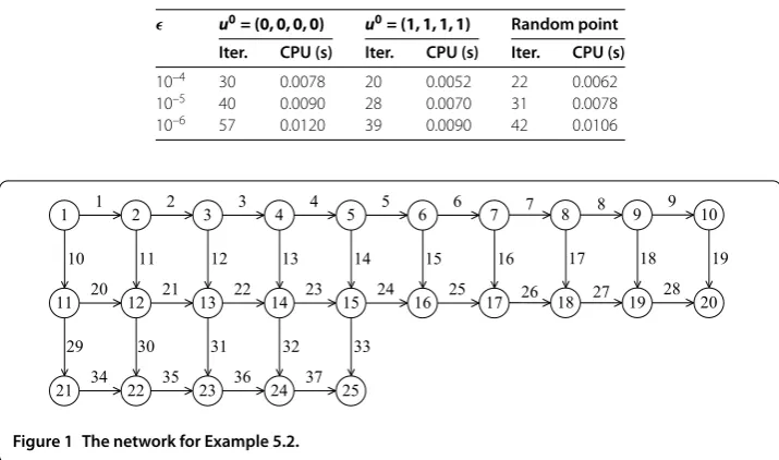
Table 1 Computational results for Example 5.1

u0= (0, 0, 0, 0) u0= (1, 1, 1, 1) Random point

Iter. CPU (s) Iter. CPU (s) Iter. CPU (s)

10–4 ₃₀ _0.0078 ₂₀ _0.0052 ₂₂ _0.0062

10–5 ₄₀ _0.0090 ₂₈ _0.0070 ₃₁ _0.0078

[image:11.595.118.476.93.304.2]

10–6 ₅₇ _0.0120 ₃₉ _0.0090 ₄₂ _0.0106

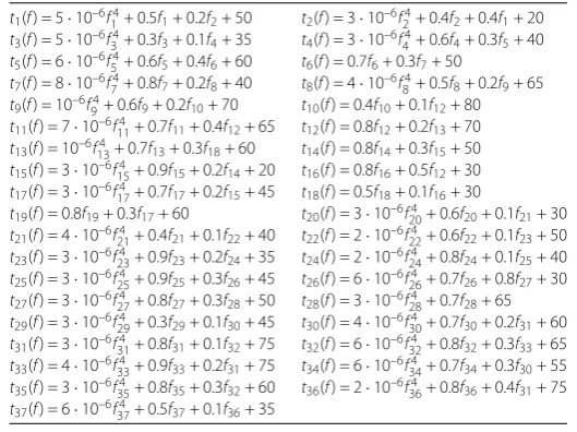
Figure 1 The network for Example 5.2.

and optimality tolerances on the performance of our algorithm. In the tests, initial points areu= (, , , ),u= (, , , ), or a random point in (, ). Optimality tolerances are = –_, _{= }– _or_{= }–_{. In our experiments, the parameter setting is}_α_{= . and}

H= .I. The associated numerical results are recorded in Table  where Iter. means the number of iterations and CPU means CPU time. The numerical results from Table  con-ﬁrm the validity and eﬃciency of our method. Moreover, we observe that the proposed algorithm is robust to the initial points.

To further showcase the performance of the proposed algorithm, we use it to solve a generic test problem, a traffic equilibrium problem with fixed demand. Now, we introduce the problem briefly.

Example . A traﬃc equilibrium problem with ﬁxed demand constraints.

The problem is always selected as a test case; for example, see [, , ]. Its network is shown in Figure  where there are  nodes,  links, and  paths. Other parameters and notations are summarized in Table .

We define variablesxpas the traffic flow of pathp. Then arc flow vectorf is calculated by the following formula:

f =ATx, dw=

p∈Pw

xp, and d=Bx.

Moreover, based on the link travel cost vector denoted byt(f) ={ta,a∈L}whose expres-sions are given in Table , the travel cost vectorθcan be formulated as follows:

θ=At(f) =AtATx.

Hence, the problem is converted to a variational inequality as

x–x∗Tθ(x)≥, ∀x∈S,

(12)

[image:12.595.122.472.96.257.2]

Table 2 Parameter setting and notations for the network

Parameter Description Value

a Link connecting two nodes

L Link set

fa Link ﬂow on linka

f Arc ﬂow vector

p Path

ω O/D pairs {ω1= (1, 20),ω2= (1, 25),ω3= (1, 24),ω4= (2, 20),

ω5= (3, 25),ω6= (11, 25)}

Pω Set of the paths connecting O/D pairω

dω Traﬃc amount between O/D pairω d1= 10,d2= 20,d3= 20,d4= 55,d5= 100,d6= 30 d O/D pair traﬃc amount vector

A Path-arc incidence matrix A(i,j) = 1 if theith path contains linkj, otherwise

A(i,j) = 0,A∈R55×37

B Path-O/D pair incidence matrix B(i,j) = 1 if theith O/D pair contains pathj, otherwiseB(i,j) = 0,B∈R6×55

Table 3 The link cost functionta(f) for Example 5.2

t1(f) = 5·10–6f14+ 0.5f1+ 0.2f2+ 50 t2(f) = 3·10–6f24+ 0.4f2+ 0.4f1+ 20 t3(f) = 5·10–6f34+ 0.3f3+ 0.1f4+ 35 t4(f) = 3·10–6f44+ 0.6f4+ 0.3f5+ 40 t5(f) = 6·10–6f54+ 0.6f5+ 0.4f6+ 60 t6(f) = 0.7f6+ 0.3f7+ 50

t7(f) = 8·10–6f74+ 0.8f7+ 0.2f8+ 40 t8(f) = 4·10–6f84+ 0.5f8+ 0.2f9+ 65 t9(f) = 10–6f94+ 0.6f9+ 0.2f10+ 70 t10(f) = 0.4f10+ 0.1f12+ 80 t11(f) = 7·10–6f114 + 0.7f11+ 0.4f12+ 65 t12(f) = 0.8f12+ 0.2f13+ 70 t13(f) = 10–6f134 + 0.7f13+ 0.3f18+ 60 t14(f) = 0.8f14+ 0.3f15+ 50 t15(f) = 3·10–6f154 + 0.9f15+ 0.2f14+ 20 t16(f) = 0.8f16+ 0.5f12+ 30 t17(f) = 3·10–6f174 + 0.7f17+ 0.2f15+ 45 t18(f) = 0.5f18+ 0.1f16+ 30

t19(f) = 0.8f19+ 0.3f17+ 60 t20(f) = 3·10–6f204 + 0.6f20+ 0.1f21+ 30 t21(f) = 4·10–6f214 + 0.4f21+ 0.1f22+ 40 t22(f) = 2·10–6f224 + 0.6f22+ 0.1f23+ 50 t23(f) = 3·10–6f234 + 0.9f23+ 0.2f24+ 35 t24(f) = 2·10–6f244 + 0.8f24+ 0.1f25+ 40 t25(f) = 3·10–6f254 + 0.9f25+ 0.3f26+ 45 t26(f) = 6·10–6f264 + 0.7f26+ 0.8f27+ 30 t27(f) = 3·10–6f274 + 0.8f27+ 0.3f28+ 50 t28(f) = 3·10–6f284 + 0.7f28+ 65 t29(f) = 3·10–6f294 + 0.3f29+ 0.1f30+ 45 t30(f) = 4·10–6f304 + 0.7f30+ 0.2f31+ 60 t31(f) = 3·10–6f314 + 0.8f31+ 0.1f32+ 75 t32(f) = 6·10–6f324 + 0.8f32+ 0.3f33+ 65 t33(f) = 4·10–6f334 + 0.9f33+ 0.2f31+ 75 t34(f) = 6·10–6f344 + 0.7f34+ 0.3f30+ 55 t35(f) = 3·10–6f354 + 0.8f35+ 0.3f32+ 60 t36(f) = 2·10–6f364 + 0.8f36+ 0.4f31+ 75 t37(f) = 6·10–6f374 + 0.5f37+ 0.1f36+ 35

We implement our algorithm for this problem. First, the decision variable vectorxis partitioned into three parts,

x=

⎛ ⎜ ⎝

x

x

x ⎞ ⎟ ⎠,

wherex∈R,x∈R, andx∈R. Subsequently, matricesA,B, andθare partitioned,

respectively, as follows:

A=

⎛ ⎜ ⎝

A

A

A ⎞ ⎟

⎠, B= (B B B), and θ= ⎛ ⎜ ⎝ θ θ θ

⎞ ⎟ ⎠,

whereA∈R×,A∈R×,A∈R×,B∈R×,B∈R×,B∈R×, andθ

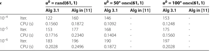
[image:12.595.165.430.290.488.2]

(13)

[image:13.595.118.479.99.188.2]

Table 4 Computational results for Example 5.2

u0=rand(61, 1) u0= 50∗ones(61, 1) u0= 100∗ones(61, 1)

Alg 3.1 Alg in [11] Alg 3.1 Alg in [11] Alg 3.1 Alg in [11]

10–4 _Iter. ₁₂₂ ₁₆₀ ₁₄₆ _- ₁₅₃

-CPU (s) 0.1560 0.1872 0.1092 - 0.1248

-10–5 _Iter. ₁₅₃ ₁₇₇ ₁₆₈ _- ₁₇₅

-CPU (s) 0.1716 0.2340 0.1404 - 0.1560

-10–6 _Iter. ₁₈₃ ₁₉₆ ₁₉₀ _- ₁₉₇

-CPU (s) 0.2028 0.2496 0.1872 - 0.2028

-Based on the above partitions, the resulting traﬃc problem is as follows:

x–x∗ T

θ(x)≥, ∀x∈S, (.)

x–x∗ T

θ(x)≥, ∀x∈S, (.)

and

x–x∗ T

θ(x)≥, ∀x∈S, (.)

whereS={(x,x,x)|Bx+Bx+Bx=d,x≥,x≥,x≥}.

In order to show the efficiency and effectiveness of our algorithm, we conduct numer-ical experiments on the performance of the proposed algorithm and the parallel split-ting augmented Lagrangian method in [] since both methods are used for a one-leader-three-follower game. The performance of the two algorithms with different initial points (u=rand(, ),u= ∗ones(, ), andu= ∗ones(, )) and optimality tolerance (= –_,_{= }–_{, and}_{= }–_{) for the traffic equilibrium problem with fixed demand}

constraints (Example .) is stated in Table . Here, Alg means algorithm and ’-’ means failure. In these tests, the common parameters of the two methods are the same, that is,

H=βI, whereβ= . andIis the identity matrix, and the maximum number of iterations

is ,.

The numerical results from Table  demonstrate the preference of our algorithm over the algorithm in [] since both the number of iterations and the CPU time of our algo-rithm are smaller than those of the algoalgo-rithm in [] for a random initial point and our algorithm can solve the problem while the algorithm in [] fails to solve it for other initial points. The results verify the eﬃciency and eﬀectiveness of the proposed algorithm again.

6 Conclusion

The system (.)-(.) can be considered as a mathematical formulation of a one-leader-m-follower Stackelberg game in which the leader constantly improves his strategy by de-termining the value ofλfrom strategy setRl_{while the}_{ith follower determines his plan}_x

i from setXibased on the value ofλ. Based on the characteristic, we design an augmented Lagrangian-based parallel splitting method to solve the system. In the method, each player can only control and improve his own decision. We establish the global convergence of the method under some suitable conditions. Finally, we conduct a computational study to demonstrate the validity and eﬃciency of our algorithm.

(14)

the condition that each player’s utility function is strongly monotone. We plan to relax the condition such that our method can be applied to more practical problems. Second, our method only serves to solve problems with a separable structure, which sounds reasonable but may not always be the case. We should improve it to solve general problems.

Competing interests

The authors declare that they have no competing interests.

Authors’ contributions

All authors contributed equally and signiﬁcantly in this paper. All authors read and approved the ﬁnal manuscript.

Acknowledgements

This work is supported by grants from the NSF of Shanxi Province (2014011006-1).

Received: 2 December 2015 Accepted: 19 March 2016

References

1. Eckstein, J, Bertsekas, DP: On the Douglas-Rachford splitting method and the proximal point algorithm for maximal monotone operators. Math. Program.55, 293-318 (1992)

2. Fukushima, M: Application of the alternating direction method of multipliers to separable convex programming problems. Comput. Optim. Appl.1, 93-111 (1992)

3. Chen, G, Teboulle, M: A proximal-based decomposition method for convex minimization problems. Math. Program.

64, 81-101 (1994)

4. Tseng, P: Alternating projection-proximal methods for convex programming and variational inequalities. SIAM J. Optim.7, 951-965 (1997)

5. Han, D, He, H, Yang, H, Yuan, X: A customized Douglas-Rachford splitting algorithm for separable convex minimization with linear constraints. Numer. Math.127, 167-200 (2014)

6. Hestenes, MR: Multiplier and gradient methods. J. Optim. Theory Appl.4, 303-320 (1969)

7. Gabay, D, Mercier, B: A dual algorithm for the solution of nonlinear variational problems via ﬁnite element approximations. Comput. Math. Appl.2, 17-40 (1976)

8. Esser, E: Applications of Lagrangian-based alternating direction methods and connections to split Bregman. CAM Report 09-31, UCLA (2009)

9. Lin, Z, Chen, M, Ma, Y: The augmented lagrange multiplier method for exact recovery of corrupted low-rank matrices. UILU-ENG 09-2215, UIUC (2009)

10. Yang, JF, Zhang, Y: Alternating direction algorithms for1-problems in compressive sensing. SIAM J. Sci. Comput.33, 250-278 (2011)

11. He, BS: Parallel splitting augmented Lagrangian methods for monotone structured variational inequalities. Comput. Math. Appl.42, 195-212 (2009)

12. Tao, M: Some parallel splitting methods for separable convex programming withO(1/t) convergence rate. Pac. J. Optim.10, 359-384 (2014)

13. Wang, K, Xu, L, Han, D: A new parallel splitting descent method for structured variational inequalities. J. Ind. Manag. Optim.10, 461-476 (2014)

14. Jiang, ZK, Yuan, XM: New parallel descent-like method for solving a class of variational inequalities. J. Optim. Theory Appl.145, 311-323 (2010)

15. Han, D, Yuan, X, Zhang, W: An augmented Lagrangian based parallel splitting method for separable convex minimization with applications to image processing. Math. Comput.83, 2263-2291 (2014)

16. Facchinei, F, Fischer, A, Piccialli, V: Generalized Nash equilibrium problems and Newton methods. Math. Program.117, 163-194 (2009)

17. Facchinei, F, Kanzow, C: Penalty methods for the solution of generalized Nash equilibrium problems. SIAM J. Optim.

20, 2228-2253 (2010)

18. Han, D, Zhang, H, Qian, G, Xu, L: An improved two-step method for solving generalized Nash equilibrium problems. Eur. J. Oper. Res.216, 613-623 (2012)

19. Nagurney, A, Zhang, D: Projected Dynamical Systems and Variational Inequalities with Applications. Kluwer Academic, Boston (1996)