Error analysis of variational discretization solving temperature control problems

R E S E A R C H

Open Access

Error analysis of variational discretization

solving temperature control problems

Yuelong Tang

*_{Correspondence:}

[email protected] Department of Mathematics and Computational Science, Hunan University of Science and Engineering, Yongzhou, Hunan 425100, China

Abstract

In this paper, we consider variational discretization solving temperature control problems with pointwise control constraints, where the state and the adjoint state are approximated by piecewise linear finite element functions, while the control is not directly discretized. We derivea priorierror estimates of second-order for the control, the state and the adjoint state. Moreover, we obtaina posteriorierror estimates. Finally, we present some numerical algorithms for the control problem and do some

numerical experiments to illustrate our theoretical results.

Keywords: variational discretization; finite element; optimal control problems;a priorierror estimates;a posteriorierror estimates

1 Introduction

We are interested in a material plate defined in a two-dimensional convex domainwith

a Lipschitz boundary∂. For the stateyof the material, we choose the temperature distri-bution which is maintained equal to zero along the boundary. We denote thermal radiation or positive temperature feedback due to chemical reactions by the termφ(y) (see,e.g., []) and assume that there exists a sourcef ∈L_{(). This system is governed by the following} equation:

–div(A(x)∇y(x)) +φ(y(x)) =f(x), x∈,

y(x) = , x∈∂.

The setting above suggests that we may control the temperature distributionyto come

close to a given target by acting with an additional distributed source termu, namely the control function. The corresponding optimal control problem is formulated as follows:

⎧ ⎪ ⎨ ⎪ ⎩

min_u∈K{(g(y) +h(u))dx},

–div(A(x)∇y(x)) +φ(y(x)) =f(x) +Bu(x), x∈,

y(x) = , x∈∂,

(.)

whereg(·) andh(·) are strictly convex continuous differentiable functions,h(u)→+∞as

u_L₍₎→ ∞,A(x) = (aij(x))×∈(W,∞(¯))× such that (A(x)ξ)·ξ≥c|ξ|,∀ξ∈R, f(x)∈L_{(),Bis a linear continuous operator, andKis defined by}

K=v(x)∈L() :a≤v(x)≤b, a.e.x∈ ,

whereaandbare two constants.

Optimal control problems have been extensively used in many aspects of the modern life such as social, economic, scientific and engineering numerical simulation []. Finite element approximation seems to be the most widely used method in computing optimal control problems. A systematic introduction of finite element method for PDEs and opti-mal control problems can be found in [–]. Concerning elliptic optiopti-mal control problems,

a priorierror estimates were investigated in [, ],a posteriorierror estimates based on recovery techniques have been obtained in [–],a posteriorierror estimates of resid-ual type have been derived in [–], some error estimates and superconvergence results have been established in [–], and some adaptive finite element methods can be found

in [–]. For parabolic optimal control problems, a priorierror estimates are

estab-lished in [–],a posteriorierror estimates of residual type are investigated in [, ]. Recently, error estimates of spectral method for optimal control problems have been de-rived in [, ], and numerical methods for constrained elliptic control problems with rapidly oscillating coefficients are studied in [].

For a constrained optimal control problem, the control has lower regularity than the state and the adjoint state. So most researchers considered using piecewise linear finite ele-ment functions to approximate the state and the adjoint state and using piecewise constant functions to approximate the control. They constructed a projection gradient algorithm where thea priorierror estimates of the control is first-order in [, ]. Recently, Borzì considered a second-order discretization and multigrid solution of elliptic nonlinear con-strained control problems in [], Hinze introduced a variational discretization concept for optimal control problems and deriveda priorierror estimates for the control which is second-order in [, ]. The purpose of this paper is to consider variational discretiza-tion for convex temperature control problems governed by nonlinear elliptic equadiscretiza-tions with pointwise control constraints.

In this paper, we adopt the standard notationWm,q_{() for Sobolev spaces on with}

the norm · Wm,q₍₎and seminorm| · |_Wm,q₍₎. We setH

()≡ {v∈H() :v|∂= }and

denoteWm,_{() byH}m_{(). In addition,corCdenotes a generic positive constant.}

The paper is organized as follows: In Section , we introduce a variational

discretiza-tion approximadiscretiza-tion scheme for the model problem. In Secdiscretiza-tion , we derivea priorierror

estimates. In Section , we derive sharpa posteriorierror estimates of residual type. We present some numerical algorithms and do some numerical experiments to verify our the-oretical results in the last section.

2 Variational discretization approximation for the model problem

We now consider a variational discretization approximation for the model problem (.). For ease of exposition, we setV =H

(),U=L(), · = · L₍₎, · _,= · _H₍₎,

· ,= · H₍₎and

a(y,w) =

A(x)∇y· ∇w, ∀y,w∈V,

(u,w) =

u·w, ∀u,w∈U.

It follows from the assumptions onA(x) that

Then the standard weak formula for the state equation is

a(y,w) +φ(y),w= (f+Bu,w), ∀w∈V, (.)

where we assume that the functionφ(·)∈W,∞(–R,R) for anyR> ,φ(·)≥ andφ(y)∈

L_{() for anyy∈H}_{(). Thus, the equation above has a unique solution.} Throughout the paper, we impose the following assumptions:

(A) g(·)andh(·)are Lipschitz continuous, namely,

g(y) –g(y)≤C|y–y|, ∀y,y∈L(), _hu(x

)

–hu(x)≤C|x–x|, ∀u∈K,x,x∈ ¯.

(A) There exists a positive constantmsuch that

h(u)≥m, ∀u∈K.

Then the model problem (.) can be restated as

minu∈K{

(g(y) +h(u))dx},

a(y,w) + (φ(y),w) = (f +Bu,w), ∀w∈V. (.)

It is well known (see,e.g., []) that the control problem (.) has a solution (y,u)∈V×K, and that if the pair (y,u)∈V×Kis the solution of (.), then there is an adjoint statep∈V

such that the triplet (y,p,u)∈V×V×Ksatisfies the following optimality conditions:

a(y,w) +φ(y),w= (f+Bu,w), ∀w∈V, (.)

a(q,p) +φ(y)p,q=g(y),q, ∀q∈V, (.)

h(u) +B∗p,v–u≥, ∀v∈K, (.)

whereB∗is the adjoint operator ofB.

Lemma . Suppose that assumptions(A)-(A)are satisfied.Let p∈V be the solution of

(.)-(.).Then the following equation:

hs(x)+B∗p(x) = , (.)

admits a unique solution s(x)and s(x)∈C,₍¯_).

Proof It follows fromh(u)≥m>  that (.) has a unique solution. Note thatg(y)∈

L(). From the regularity theory of patrial differential equations (see,e.g., []), we have

p(x)∈H_()∩W,().

Becauseis a two-dimension convex domain, according to embedding theorem, we get

From (A) and (.), we get

ms(x) –s(x)

≤ 



hθs(x) + ( –θ)s(x)

dθ·s(x) –s(x)

=hs(x)–hs(x)

=–B∗p(x) +B∗p(x)

≤C|x–x|.

Consequently, we complete the proof of equation (.).

We introduce the following pointwise projection operator:

[a,b]

g(x)=maxa,minb,g(x). (.)

It is clear that[a,b](·) is Lipschitz continuous with constant . As in [], it is easy to prove the following lemma.

Lemma . Let(y,p,u)and s(x)be the solutions of(.)-(.)and(.),respectively. As-sume that assumptions(A)-(A)are satisfied.Then

u(x) =[a,b]

s(x). (.)

Remark . We should point out that (.) and (.) are equivalent. This theory can be used to more complex situation, for example,Kis characterized by a bound on the integral onuover, namely,u(x)dx≥, we have similar results.

LetTh _{be a regular triangulation of, such that}¯ ₌

τ∈Thτ¯. Leth=max_τ∈Th{hτ},

wherehτdenotes the diameter of the elementτ. Associated withThis a finite dimensional

subspaceSh_ofC(¯_{), such thatχ|}

τ are polynomials of m-order (m≥) for allχ∈Shand

τ ∈Th_{. LetV}h_={v

h∈Sh:vh|∂= }. It is easy to see thatVh⊂V.

Then a possible variational discretization approximation scheme of (.) is as follows:

minuh∈K{

(g(yh) +h(uh))dx},

a(yh,wh) + (φ(yh),wh) = (f +Buh,wh), ∀wh∈Vh.

(.)

It is well known (see,e.g., []) that control problem (.) has a solution (yh,uh)∈Vh×K,

and that if the pair (yh,uh)∈Vh×Kis the solution of (.), then there is an adjoint state

ph∈Vhsuch that the triplet (yh,ph,uh)∈Vh×Vh×Ksatisfies the following optimality

conditions:

a(yh,wh) +

φ(yh),wh

= (f+Buh,wh), ∀wh∈Vh, (.)

a(qh,ph) +

φ(yh)ph,qh

=g(yh),qh

, ∀qh∈Vh, (.)

h(uh) +B∗ph,v–uh

≥, ∀v∈K. (.)

Lemma . Suppose that assumptions(A)-(A)are satisfied.Let(yh,ph,uh)be the

solu-tion of(.)-(.),and sh(x)is the solution of the following equation:

hsh(x)

+B∗ph(x) = . (.)

Then we have

uh(x) =[a,b]

sh(x)

. (.)

Remark . In many applications, the objective functional is uniform convex near the so-lutionu, which is assumed in many studies on numerical methods of the problem, see, for example, [, ]. In this paper, we assumed thatg(·) andh(·) are strictly convex continu-ous differentiable functions, for instance,h(u) = α_u_{, which is frequently met, then the} exact solution of the variational inequality (.) isuh(x) =max(a,min(b, –αB∗ph(x))), and

for numerically solving the problem, we can replaceuh(x) bymax(a,min(b, –αB∗ph(x))) in

our program.

3 A priorierror estimates

We now derive a priorierror estimates of the variational discretization approximation

scheme. Just for ease of exposition, let

J(u) =

g(y) +h(u)dx,

andJ(u) is the Fréchet derivative ofJ(u) atu. Similarly to (.)-(.), we can prove that

J(u),v=h(u) +B∗p,v, ∀v∈K,

J(uh),v

=h(uh) +B∗p(uh),v

, ∀v∈K,

wherep(uh) satisfies the following system:

ay(uh),w

+φy(uh)

,w= (f +Buh,w), ∀w∈V, (.)

aq,p(uh)

+φy(uh)

p(uh),q

=gy(uh)

,q, ∀q∈V. (.)

Letπh:C(¯)→Vhbe the standard Lagrange interpolation operator such that for any

v∈C₍¯_),π

hv(Pi) =v(Pi) for allPi∈P, wherePis the vertex set associated with the

tri-angulationTh, andnis the dimension of the domain, we have the following result:

Lemma .[] Letπh be the standard Lagrange interpolation operator.For m= or,

q>n_ and∀v∈W,q_{(),we have}

|v–πhv|Wm,q₍₎≤Ch–m|v|_W,q₍₎.

Lemma . Let(yh,ph,uh)and(y(uh),p(uh))be the solutions of(.)-(.)and(.)-(.),

respectively. Assume that p(uh),y(uh)∈H()andφ(·)is locally Lipschitz continuous.

Then there exists a constant C independent of h such that

Proof Fromφ(·)≥, (.), (.) and embedding theoremvL₍₎≤Cv_H₍₎, we have

cp(uh) –ph

 ,

≤ap(uh) –ph,p(uh) –ph

+φy(uh)

p(uh) –ph

,p(uh) –ph

=ap(uh) –πhp(uh),p(uh) –ph

+φy(uh)

p(uh) –ph

,p(uh) –πhp(uh)

+gy(uh)

–g(yh),πhp(uh) –ph

+φ(yh) –φ

y(uh)

ph,πhp(uh) –ph

≤Cp(uh) –ph_,p(uh) –πhp(uh)_,+Cy(uh) –yhπhp(uh) –ph

+Cφy(uh)p(uh) –ph_L₍₎p(uh) –πhp(uh)_L₍₎ +Cy(uh) –yhphL₍₎π_hp(u_h) –p_h

L₍₎

≤C(δ)p(uh) –πhp(uh)



,+C(δ)y(uh) –yh



+Cδp(uh) –ph_,+πhp(uh) –ph_,

≤C(δ)p(uh) –πhp(uh)



,+C(δ)y(uh) –yh



+Cδp(uh) –ph



,. (.)

Note thatp(uh)∈H(), by using Lemma ., we obtain

_p(uh) –ph_,≤Cp(uh) –πh

p(uh)_,+Cy(uh) –yh

≤Chp(uh)_,+Cy(uh) –yh

≤Ch+Cy(uh) –yh. (.)

Similarly, we can prove that

y(uh) –yh_,≤Chy(uh)_,≤Ch. (.)

Then (.) follows from (.)-(.).

In order to derive sharpa prioriestimates, we introduce the following auxiliary prob-lems:

–divA∗∇ξ+ξ=F, in,ξ|∂= , (.)

–div(A∇ζ) +φy(uh)

ζ=F, in,ζ|∂= , (.)

where

=

_φ(y(u h))–φ(yh)

y(uh)–yh , y(uh)=yh, φ(yh), y(uh) =yh.

From the regularity estimates (see,e.g., []), we obtain

Lemma . Let (yh,ph,uh) be the solution of (.)-(.). Suppose that y(uh),p(uh)∈

H_{()andφ(·)is locally Lipschitz continuous.Then there exists a constant C} indepen-dent of h such that

y(uh) –yh+p(uh) –ph≤Ch. (.)

Proof LetF=y(uh) –yhandξh=πhξ. We have

y(uh) –yh



=ay(uh) –yh,ξ

+ξ,y(uh) –yh

=ay(uh) –yh,ξ–ξh

+ξ,y(uh) –yh

–φy(uh)

–φ(yh),ξh

=ay(uh) –yh,ξ–ξh

+φy(uh)

–φ(yh),ξ–ξh

≤Cy(uh) –yh_,ξ–ξh,+Cy(uh) –yhξ–ξh

≤Cy(uh) –yh_,ξ–ξh,. (.)

Note that

ξ–ξh,≤Chξ,≤Chy(uh) –yh. (.)

Thus,

y(uh) –yh≤Chy(uh) –yh_,≤Ch. (.)

Similarly, letF=p(uh) –phandζh=πhζ, we obtain

_{p(uh) –ph≤Ch}_{. (.)}

From (.) and (.), we get (.).

Lemma . Let(y,p,u)and(yh,ph,uh)be the solutions of(.)-(.)and(.)-(.),

re-spectively.Assume that all the conditions in Lemma.are valid.Then there exists a con-stant C independent of h such that

u–uh ≤Ch. (.)

Proof It is clear that

J(v) –J(u),v–u≥cv–u, ∀v,u∈K. (.)

By using (.) and (.), we have

cu–uh≤

J(u) –J(uh),u–uh

=h(u) +B∗p,u–uh

–h(uh) +B∗p(uh),u–uh

≤–h(uh) +B∗ph,u–uh

+B∗ph–B∗p(uh),u–uh

≤B∗ph–B∗p(uh),u–uh

≤Cph–p(uh)u–uh. (.)

From (.) and (.), we derive (.).

Now we combine Lemmas .-. to come up with the following main result.

Theorem . Let(y,p,u)and(yh,ph,uh)be the solutions of(.)-(.)and(.)-(.),

respectively.Assume that all the conditions in Lemmas.-.are valid.Then we have

u–uh+y–yh+p–ph ≤Ch. (.)

Proof Note that

p–ph ≤p–p(uh)+p(uh) –ph, (.)

y–yh ≤y–y(uh)+y(uh) –yh. (.)

From (.)-(.), (.)-(.) and the regularity estimates, we have

p–p(uh)≤p–p(uh)_,≤Cy–y(uh), (.)

y–y(uh)≤y–y(uh)_,≤Cu–uh. (.)

Then, (.) follows from (.), (.) and (.)-(.).

4 A posteriorierror estimates

We now derivea posteriorierror estimates for the variational discretization approximation scheme. The following lemmas are very important in derivinga posteriorierror estimates of residual type.

Lemma .[] ∀v∈W,q_{(), ≤q<∞,}

vW,q_(∂τ)≤C

h–



q

τ vW,q_(τ)+h –_q

τ |v|W,q_(τ)

. (.)

Lemma . Let(y,p,u)and(yh,ph,uh)be the solutions of(.)-(.)and(.)-(.),

re-spectively.Then we have

u–uh ≤Cph–p(uh), (.)

Proof It follows from (.) and (.) that

cu–uh≤

J(u),u–uh

–J(uh),u–uh

≤–J(uh),u–uh

= –h(uh) +B∗ph,u–uh

+B∗ph–B∗p(uh),u–uh

≤C(δ)ph–p(uh)



+δu–uh. (.)

Letδbe small enough, then (.) follows from (.).

Lemma . Let(yh,ph,uh)and(y(uh),p(uh))be the solutions of(.)-(.)and(.)-(.),

respectively.Assume thatφ(·)is locally Lipschitz continuous.Then there exists a positive constant C independent of h such that

yh–y(uh)_,+ph–p(uh)_,≤C

η_+η_, (.)

where

η_=

τ∈Th h_τ

τ

g(yh) +div

A∗∇ph

–φ(yh)ph



dx+

l∩∂=∅

hl

l

A∗∇ph·n

 ds,

η_=

τ∈Th h_τ

τ

div(A∇yh) –φ(yh) +f+Buh



dx+

l∩∂=∅

hl

l

[A∇yh·n]ds,

where hlis the size of the face l=τ¯l∩ ¯τl,andτl,τlare two neighboring elements inTh,

[A∇yh·n]l,and[A∗∇ph·n]lare the A-normal and A∗-normal derivative jumps over the

interior face l,respectively,defined by

[A∇yh·n]l= (A∇yh|τ_l–A∇yh|τ_l)·n,

A∗∇ph·n

l=

A∗∇ph|τ_l–A∗∇ph|τ_l

·n,

wherenis the normal vector on l=τ

l ∩τloutwardsτl.For later convenience,we defined

[A∇yh·n]l= and[A∗∇ph·n]l= when l⊂∂.

Proof Letep_=p

h–p(uh) andepI =πhep, it follows from the Green formula, embedding

theoremv_L₍₎≤Cv_H₍₎, Lemma ., (.) and (.) that

cph–p(uh)_,

≤aep,ph–p(uh)

+φy(uh)

ph–p(uh)

,ep

=aep–ep_I,ph–p(uh)

+φ(yh)ph–φ

y(uh)

p(uh),ep–epI

+aep_I,ph–p(uh)

+φ(yh)ph–φ

y(uh)

p(uh),epI

+φy(uh)

ph–φ(yh)ph,ep

=

τ∈Th

τ

g(yh) +div

A∗∇ph

–φ(yh)ph

ep_I –epdx+g(yh) –g

y(uh)

+

τ∈Th

∂τ

A∗∇ph·n

ep–ep_Ids+φy(uh)

ph–φ(yh)ph,ep

≤Cη_+C(δ)yh–y(uh)_,+δph–p(uh)_,. (.)

Similarly, we obtain

cyh–y(uh)

 ,

≤ayh–y(uh),ey

+φ(yh) –φ

y(uh)

,ey

=A∇yh–y(uh)

,∇ey–ey_I+φ(yh) –φ

y(uh)

,ey–ey_I

=

τ∈Th

τ

div(A∇yh) –φ(yh) +f+Buh

ey_I–ey_dx+

τ∈Th

∂τ

(A∇yh·n)

ey_–ey

I

ds

≤C(δ)η_+δyh–y(uh)



,. (.)

From (.) and (.), we derive (.).

Theorem . Let(y,p,u)and(yh,ph,uh)be the solutions of(.)-(.)and(.)-(.),

respectively.Assume that all the conditions in Lemmas.-.are valid.Then there exists a constant C independent of h such that

u–uh+y–yh,+p–ph,≤C

η_+η_, (.)

whereηandηare defined in Lemma..

Proof Note that

p–ph,≤p–p(uh)_,+ph–p(uh)_,, (.)

y–yh,≤y–y(uh)_,+yh–y(uh),, (.)

and

p–p(uh)_,≤p–p(uh)_,≤Cy–y(uh), (.)

y–y(uh)_,≤y–y(uh),≤Cu–uh. (.)

Then (.) follows from (.), (.) and (.)-(.).

5 Numerical experiments

For a constrained optimization problem

min

u∈K⊂UJ(u),

whereJ(u) is a convex functional onUandKis a convex subset ofU, the iterative scheme reads (n= , , , . . .):

b(u_n+

,v) =b(un,v) –ρn(J _(u

n),v), ∀v∈U,

un+=PbK(un+),

whereb(·,·) is a symmetric and positive definite bilinear form, and similarly to [], the projection operatorP_Kb :U→Kis defined: For givenw∈UfindPb_Kw∈Ksuch that

bPb_Kw–w,Pb_Kw–w=min

u∈Kb(u–w,u–w).

The bilinear formb(·,·) provides a suitable precondition for the projection gradient al-gorithm. LetUh_={v

h∈L(),a≤vh≤b:vh|τ =constant,∀τ ∈Th}. For an acceptable

errortoland a fixed step sizeρn, by applying (.) to the discretized nonlinear elliptic

op-timal control problem, we introduce the following projection gradient algorithm (see,e.g., [, ]), for ease of exposition, we have omitted the subscripth.

Algorithm .(Projection gradient algorithm) Step . Initializeu;

Step . Solve the following equations:

⎧ ⎪ ⎪ ⎪ ⎪ ⎨ ⎪ ⎪ ⎪ ⎪ ⎩

b(u_n+

,v) =b(un,v) –ρn(h _(u

n) +B∗pn,v), un+_,un∈Uh,∀v∈Uh,

a(yn,w) + (φ(yn),w) = (f +Bun,w), yn∈Vh,∀w∈Vh,

a(q,pn) + (φ(yn)pn,q) = (yn–yd,q), pn∈Vh,∀q∈Vh,

un+=PbK(un+_);

(.)

Step . Calculate the iterative error:en+=un+–un;

Step . Ifen+≤tol, stop; else, go to Step .

According to the preceding analysis, we construct the following variational discretiza-tion algorithm.

Algorithm .(Variational discretization algorithm) Step . Initializeu;

Step . Solve the following equations:

⎧ ⎪ ⎪ ⎪ ⎪ ⎨ ⎪ ⎪ ⎪ ⎪ ⎩

b(u_n+

,v) =b(un,v) –ρn(h _(u

n) +B∗pn,v), un+_,un∈U,∀v∈U,

a(yn,w) + (φ(yn),w) = (f +Bun,w), yn∈Vh,∀w∈Vh,

a(q,pn) + (φ(yn)pn,q) = (yn–yd,q), pn∈Vh,∀q∈Vh,

un+=[a,b](un+_).

(.)

Step . Calculate the iterative error:en+=un+–un;

Step . Ifen+≤tol, stop; else, go to Step .

It is well known that there are four major types of adaptive finite element methods,

namely, the h-methods (mesh refinement), thep-methods (order enrichment), the r

-methods (mesh redistribution) and thehp-methods (the combination ofh-method and

p-method). For an acceptable errorTol, by usinga posteriorierror estimatorη

Algorithm .(Adaptive variational discretization algorithm)

Step . Solve the discretized optimization problem with Algorithm . on the current mesh obtain the numerical solutionu_nand calculate the error estimatorsηandη;

Step . Adjust the mesh by using estimatorsηandη, then update the numerical solu-tionu_nand obtain the new numerical solutionu_n+on new mesh;

Step . Ifu_n+–u_n ≤Tol, stop; else, go to Step .

All of the following numerical examples were solved numerically with codes developed based on AFEPack which provided a general tool of finite element approximation for PDEs. The package is freely available and the details can be found in [].

We consider the following optimal control problems:

⎧ ⎪ ⎨ ⎪ ⎩

minu∈K{

(g(y(x)) +h(u(x)))dx},

–div(A(x)∇y(x)) +φ(y(x)) =f(x) +Bu(x), x∈,

y(x) = , x∈∂,

where

gy(x)=  

y(x) –y(x) 

,

hu(x)=  

u(x) –u(x) 

,

and

K=v(x)∈L() :a≤v(x)≤b,x∈ ,

the domainis the unit square [, ]×[, ] andB=I.

Example  In the first example, we compare the convergence order ofu–uhin

Algo-rithm . with that in AlgoAlgo-rithm .. The data are as follows:

A(x) =E, φ(y) =y, a= , b= .,

p(x) = xxsin(πx)sin(πx),

y(x) =p(x),

u(x) =  +sin(πx)sin(πx),

u(x) =min.,max,u(x) –p(x)

,

f(x) = –divA(x)∇y(x)+φy(x)–u(x),

y(x) =y(x) +div

A∗(x)∇p(x)–φy(x)p(x).

The numerical results are listed in Table  and Table .

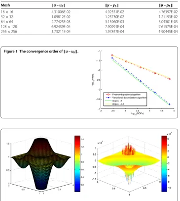
In Figure , we see clearly that in the projection gradient algorithm,u–uh=O(h),

while in the variational discretization algorithm,u–uh=O(h). In Figure , we show

Table 1 Algorithm 5.1, Example 1

Mesh u–uh y–yh p–ph

16×16 5.98051E-02 4.92490E-02 4.76241E-02 32×32 2.84008E-02 1.25725E-02 1.21182E-02 64×64 1.39765E-02 3.15952E-03 3.04294E-03 128×128 6.96692E-03 7.90942E-04 7.61570E-04 256×256 3.48077E-03 1.97800E-04 1.90445E-04

Table 2 Algorithm 5.2, Example 1

Mesh u–uh y–yh p–ph

16×16 4.31006E-02 4.92551E-02 4.76397E-02 32×32 1.09812E-02 1.25730E-02 1.21193E-02 64×64 2.77425E-03 3.15960E-03 3.04301E-03 128×128 6.92439E-04 7.90991E-04 7.61575E-04 256×256 1.73211E-04 1.97847E-04 1.90445E-04

Figure 1 The convergence order ofu–uh.

Figure 2 The exact solutionu(left) and the erroruh–u(right).

Example  In order to illustrate the reliability and efficiency of thea posteriorierror esti-mates in Theorem ., we use Algorithm . to solve this example. The data are as follows:

φ(y) =y, a= –., b= ,

A(x) =

Table 3 Numerical results, Example 2.

Mesh Nodes Sides Elements Dofs u–uh

Uniform mesh 513 1456 944 513 6.19419E-02 Adaptive mesh 145 392 248 145 6.04841E-02

Figure 3 The exact solutionu(left) and the erroruh–u(right).

p(x) =

sin(πx)sin(πx), x+x≥,

sin(πx)sin(πx), x+x< ,

y(x) =p(x),

u(x) = ,

u(x) =min,max–.,u(x) –p(x)

,

f(x) = –divA(x)∇y(x)+φy(x)–u(x),

y(x) =y(x) +div

A∗(x)∇p(x)–φy(x)p(x).

The numerical results based on adaptive mesh and uniform mesh are presented in Ta-ble . In Figure , we show the profiles of the exact solutionualongside the solution error. From Table , it is clear that the adaptive mesh generated via the error indicators in Theo-rem . are able to save substantial computational work, in comparison with the uniform mesh. Our numerical results confirm our theoretical results.

Competing interests

The author declares that he has no competing interests.

Acknowledgements

This work is supported by the Scientific Research Project of Department of Education of Hunan Province (13C338). Received: 23 March 2013 Accepted: 10 September 2013 Published:07 Nov 2013

References

1. Pao, C: Nonlinear Parabolic and Elliptic Equations. Plenum Press, New York (1992)

2. Lions, J: Optimal Control of Systems Governed by Partial Differential Equations. Springer, Berlin (1971) 3. Ciarlet, P: The Finite Element Method for Elliptic Problems. North-Holland, Amsterdam (1978) 4. He, BS: Solving a class of linear projection equations. Numer. Math.68, 71-80 (1994) 5. Kufner, A, John, O, Fucik, S: Function Spaces. Nordhoff, Leyden (1977)

6. Ladyzhenskaya, O, Urlatseva, H: Linear and Quasilinear Elliptic Equations. Academic Press, New York (1968) 7. Lions, J, Magenes, E: Non Homogeneous Boundary Value Problems and Applications. Springer, Berlin (1972) 8. Neittaanmaki, P, Tiba, D: Optimal Control of Nonlinear Parabolic Systems: Theory, Algorithms and Applications.

9. Arada, N, Casas, E, Tröltzsch, F: Error estimates for the numerical approximation of a semilinear elliptic control problem. Comput. Optim. Appl.23, 201-229 (2002)

10. Liu, W, Yan, N: Adaptive Finite Element Methods for Optimal Control Governed by PDEs. Science Press, Beijing (2008) 11. Li, R, Liu, W, Yan, N:A posteriorierror estimates of recovery type for distributed convex optimal control problems. J. Sci.

Comput.33, 155-182 (2007)

12. Liu, H, Yan, N: Recovery type superconvergence anda posteriorierror estimates for control problems governed by Stokes equations. J. Comput. Appl. Math.209, 187-207 (2007)

13. Yan, N:A posteriorierror estimates of gradient recovery type for FEM of optimal control problem. Adv. Comput. Math. 19, 323-336 (2003)

14. Ainsworth, M, Oden, JT: A Posteriori Error Estimation in Finite Element Analysis. Wiley, New York (2000)

15. Babuška, I, Strouboulis, T, Upadhyay, CS, Gangaraj, SK:A posterioriestimation and adaptive control of the pollution error in the h-version of the finite element method. Int. J. Numer. Methods Eng.38(24), 4207-4235 (1995)

16. Carstensen, C, Verfürth, R: Edge residuals dominatea posteriorierror estimates for low order finite element methods. SIAM J. Numer. Anal.36(5), 1571-1587 (1999)

17. Hintermüller, M, Hoppe, RHW, Iliash, Y, Lieweg, M: Ana posteriorierror analysis of adaptive finite element methods for distributed elliptic control problems with control constraints. ESAIM Control Optim. Calc. Var.14(3), 540-560 (2008) 18. Hintermüller, M, Hoppe, RHW: Goal-oriented adaptivity in control constrained optimal control of partial differential

equations. SIAM J. Control Optim.47(3), 1721-1743 (2008)

19. Liu, W, Yan, N:A posteriorierror estimates for distributed convex optimal control problems. Adv. Comput. Math.15, 285-309 (2001)

20. Liu, W, Yan, N:A posteriorierror estimates for control problems governed by nonlinear elliptic equations. Appl. Numer. Math.47, 173-187 (2003)

21. Veeser, A: Efficient and reliablea posteriorierror estimators for elliptic obstacle problems. SIAM J. Numer. Anal.39(1), 146-167 (2001)

22. Verfurth, R: A Review of Posteriori Error Estimation and Adaptive Mesh Refinement. Wiley, London (1996)

23. Brandts, J: Superconvergence anda posteriorierror estimation for triangular mixed finite elements. Numer. Math.68, 311-324 (1994)

24. Chen, Y, Dai, Y: Superconvergence for optimal control problems governed by semi-linear elliptic equations. J. Sci. Comput.39, 206-221 (2009)

25. Chen, Y, Liu, B: Error estimates and superconvergence of mixed finite element for quadratic optimal control. Int. J. Numer. Anal. Model.3, 311-321 (2006)

26. Xing, X, Chen, Y:L∞-error estimates for general optimal control problem by mixed finite element methods. Int. J. Numer. Anal. Model.5(3), 441-456 (2008)

27. Zhang, Z, Zhu, JZ: Analysis of the superconvergent patch recovery technique anda posteriorierror estimator in the finite element method (I). Comput. Methods Appl. Math.123, 173-187 (1995)

28. Becker, R, Kapp, H, Rannacher, R: Adaptive finite element methods for optimal control of partial differential equations: basic concept. SIAM J. Control Optim.39(1), 113-132 (2000)

29. Hoppe, RHW, Kieweg, M: Adaptive finite element methods for mixed control-state constrained optimal control problems for elliptic boundary value problems. Comput. Optim. Appl.46, 511-533 (2010)

30. Li, R, Liu, W, Ma, H, Tang, T: Adaptive finite element approximation for distributed elliptic optimal control problems. SIAM J. Control Optim.41(5), 1321-1349 (2002)

31. Vexler, B, Wollner, W: Adaptive finite elements for elliptic optimization problems with control constraints. SIAM J. Control Optim.47(1), 509-534 (2008)

32. Alt, W, Mackenroth, U: Convergence of finite element approximation to state constrained convex parabolic boundary control problems. SIAM J. Control Optim.27, 718-736 (1989)

33. Chen, Y, Lu, Z: Error estimates for quadratic parabolic optimal control problems by fully discrete mixed finite element methods. Finite Elem. Anal. Des.46(11), 957-965 (2010)

34. Chen, Y, Yang, J:A posteriorierror estimation for a fully discrete discontinuous Galerkin approximation to a kind of singularly perturbed problems. Finite Elem. Anal. Des.43(10), 757-770 (2007)

35. Liu, W, Yan, N:A posteriorierror estimates for optimal control problems governed by parabolic equations. Numer. Math.93, 497-521 (2003)

36. Xiong, C, Li, Y:A posteriorierror estimates for optimal distributed control governed by the evolution equations. Appl. Numer. Math.61, 181-200 (2011)

37. Chen, Y, Huang, Y, Yi, N:A posteriorierror estimates of spectral method for optimal control problems governed by parabolic equations. Sci. China Ser. A51(8), 1376-1390 (2008)

38. Chen, Y, Yi, N, Liu, W: A legendre-Galerkin spectral method for optimal control problems governed by elliptic equations. SIAM J. Numer. Anal.46(5), 2254-2275 (2008)

39. Chen, Y, Tang, Y: Numerical methods for constrained elliptic optimal control problems with rapidly oscillating coefficients. East Asian J. Appl. Math.1, 235-247 (2011)

40. Borzì, A: High-order discretization and multigrid solution of elliptic nonlinear constrained control problems. J. Comput. Appl. Math.200, 67-85 (2005)

41. Hinze, M: A variational discretization concept in control constrained optimization: the linear-quadratic case. Comput. Optim. Appl.30, 45-63 (2005)

42. Hinze, M, Yan, N, Zhou, Z: Variational discretization for optimal control governed by convection dominated diffusion equations. J. Comput. Math.27, 237-253 (2009)

43. Liu, W, Tiba, D: Error estimates for the finite element approximation of a class of nonlinear optimal control problems. Numer. Funct. Anal. Optim.22, 953-972 (2001)

10.1186/1029-242X-2013-450