A regularized alternating direction method of multipliers for a class of nonconvex problems

R E S E A R C H

Open Access

A regularized alternating direction method

of multipliers for a class of nonconvex

problems

Jin Bao Jian

_{, Ye Zhang}

_{and Mian Tao Chao}

*_{Correspondence:}

[email protected]

1_{College of Mathematics and} Information Science, Guangxi University, Nanning, China Full list of author information is available at the end of the article

Abstract

In this paper, we propose a regularized alternating direction method of multipliers (RADMM) for a class of nonconvex optimization problems. The algorithm does not require the regular term to be strictly convex. Firstly, we prove the global

convergence of the algorithm. Secondly, under the condition that the augmented Lagrangian function satisfies the Kurdyka–Łojasiewicz property, the strong convergence of the algorithm is established. Finally, some preliminary numerical results are reported to support the efficiency of the proposed algorithm.

Keywords: Nonconvex optimization problems; Alternating direction method of multipliers; Kurdyka–Łojasiewicz property; Convergence

1 Introduction

In this paper, we consider the following nonconvex optimization problem

min f(x) +g(Ax), (1)

wheref :Rn_{→R∪ {+∞} is a proper lower semicontinuous function,g:R}m_{→R is a}

continuous differentiable function with∇gLipschitz continuous and modulusL> 0, while A∈Rm×n_{is a given matrix. When the functionsf andgare convex, the problem (1) can}

be transformed into the split feasibility problem [1,2]. Problem (1) is equivalent to the following constraint optimization problem:

min f(x) +g(y),

s.t.Ax–y= 0. (2)

The augmented Lagrangian function of (2) is defined as follows:

Lβ(x,y,λ) =f(x) +g(y) –λ,Ax–y+

β

2 Ax–y

2_{, (3)}

whereλ∈Rm_{is the Lagrangian parameter andβ> 0 is the penalty parameter.}

The alternating direction method of multipliers (ADMM) was first proposed by Gabay and Mercier in 1970s, which is an effective algorithm for solving the two-block convex problems [3]. The iterative scheme of the classic ADMM for problem (2) is as follows:

⎧ ⎪ ⎪ ⎨ ⎪ ⎪ ⎩

xk+1_{∈arg min{L}

β(x,yk,λk)}, yk+1_{∈arg min{L}

β(xk+1,y,λk)},

λk+1_=λk_–β(Axk+1_–yk+1_).

(4)

Iff,gare convex functions, then the convergence of ADMM is well-understood and there are some recent convergence rate analysis results [4–8]. However, when the objective func-tion is nonconvex, ADMM does not necessarily converge. Recently, some scholars have proposed various improved ADMM for nonconvex problems, and analyzed their conver-gence [9–15]. In particular, Guo et al. [16,17] analyzed the strong convergence of classical ADMM for the nonconvex optimization problem of (2). Wang et al. [12,14] studied the convergence of the Bregman ADMM for the nonconvex optimization problems, where they need the augmented Lagrangian function with respect toxor the Bregman distance in thex-subproblem to be strongly convex.

The first formula of (4) has the following structure:

min

f(x) +gyk– λk,Ax–yk+β 2Ax–y

k2

. (5)

WhenAis not the identity matrix, the above problem may not be easy. Regularization is a popular technique to simplify the optimization problems [12,14,18]. For example, the regular term1₂ x–xk 2

Gcould be added to the above problem (5), whereGis a symmetric

semidefinite matrix. Specifically, whenG=αI–βAA, problem (5) is converted into the following form:

min

f(x) +α 2x–b

k2

, (6)

with a certain knownbk_∈Rn_{. Since the first formula of (4) has the form of (6) withα= 1,}

this paper considers the following regularized ADMM (in short, RADMM) for problem (2):

⎧ ⎪ ⎪ ⎨ ⎪ ⎪ ⎩

xk+1∈arg min{Lβ(x,yk,λk) +1₂ x–xk 2_G}, yk+1_{∈arg min{L}

β(xk+1,y,λk)},

λk+1=λk–β(Axk+1_–yk+1_),

(7)

whereGis a symmetric semidefinite matrix, x 2

G:=xGx.

The framework of this paper is as follows. In Sect.2, we present some preliminary ma-terials that will be used in this paper. In Sect.3, we prove the convergence of algorithm (7). In Sect.4, we report some numerical results. In Sect.5, we draw some conclusions.

2 Preliminaries

For a vectorx= (x1,x2, . . . ,xn)∈Rn, we let x = (

n i=1x2i)

1

2_{, x} 1₌n

i=1|xi|, and x 1 2 = (n_i=1|xi|

1

matrix. For a subsetS⊆Rn_{and a pointx∈R}n_{, ifSis nonempty, letd(x,S) =inf}

y∈S y–x .

WhenS=∅, we setd(x,S) = +∞for allx. A functionf :Rn→(–∞, +∞] is said to be proper, if there exists at least onex∈Rn_{such thatf(x) < +∞. The effective domain off is}

defined throughdomf ={x∈Rn_{|f(x) < +∞}.}

Definition 2.1([19]) The functionf :Rn_{→R∪ {+∞}is lower semicontinuous atx, if¯}

f(x)¯ ≤lim infx→¯xf(x). Iff is lower semicontinuous at every pointx∈Rn, thenf is called a

lower semicontinuous function.

Definition 2.2([19]) Letf:Rn_{→R∪ {+∞}be a proper lower semicontinuous function.}

(i) The Fréchet subdifferential, or regular subdifferential, off atx∈domf, denoted by ˆ

∂f(x), is the set of all elementsu∈Rn_{which satisfy}

ˆ

∂f(x) =

u∈Rnlim y=xyinf→x

f(y) –f(x) –u,y–x y–x ≥0

,

whenx∈/domf, let∂ˆf(x) =∅;

(ii) The limiting-subdifferential, or simply the subdifferential, off atx∈domf, denoted by∂f(x), is defined as

∂f(x) =u∈Rn| ∃xk→x,fxk→f(x),uk∈ ˆ∂fxk→u,k→ ∞.

Proposition 2.1([20]) Let f :Rn_{→R∪ {+∞}be a proper lower semicontinuous function,}

then

(i) ∂ˆf(x)⊆∂f(x)for eachx∈Rn,where the first set is closed and convex while the second one is only closed;

(ii) Letuk_∈∂f(xk_)andlim

k→∞(xk,uk) = (x,u),thenu∈∂f(x); (iii) A necessary condition forx∈Rn_{to be a minimizer off is}

0∈∂f(x); (8)

(iv) Ifg:Rn_{→Ris continuously differentiable,then∂(f+g)(x) =∂f(x) +∇g(x)for any}

x∈domf.

A point that satisfies (8) is called a critical point or a stationary point. The set of critical points off is denoted by critf.

Lemma 2.1([21]) Suppose that H(x,y) =f(x) +g(y),where f :Rn_{→R∪ {+∞} and g:}

Rm→R are proper lower semicontinuous functions,then

∂H(x,y) =∂xH(x,y)×∂yH(x,y) =∂f(x)×∂g(y),

for all(x,y)∈domH=domf×domg.

Lemma 2.2([22]) Let function h:Rn_{→R be continuously differentiable and its gradient}

∇h be Lipschitz continuous with modulus L> 0,then

h(y) –h(x) – ∇h(x),y–x≤L 2 y–x

2_{, for all x,y∈R}n_.

Definition 2.3 We say that (x∗,y∗,λ∗) is a critical point of the augmented Lagrangian

functionLβ(·) of (2) if it satisfies

⎧ ⎪ ⎪ ⎨ ⎪ ⎪ ⎩

Aλ∗∈∂f(x∗), ∇g(y∗) =λ∗, Ax∗–y∗= 0.

(9)

Obviously, (2) is equivalent to 0∈∂Lβ(x∗,y∗,λ∗).

Definition 2.4([21] (Kurdyka–Łojasiewicz property)) Letf :Rn_{→R∪ {+∞}be a proper}

lower semicontinuous function. If there existη∈(0, +∞], a neighborhoodU ofx, and aˆ concave functionϕ: [0,η)→R+satisfying the following conditions:

(i) ϕ(0) = 0;

(ii) ϕis continuously differentiable on(0,η)and continuous at 0; (iii) ϕ(s) > 0for alls∈(0,η);

(iv) ϕ(f(x) –f(x))d(0,ˆ ∂f(x))≥1, for allx∈U∩[f(x) <ˆ f(x) <f(x) +ˆ η], thenf is said to have the Kurdyka–Łojasiewicz (KL) property atx.ˆ

Lemma 2.3([23] (Uniform KL property)) LetΦη be the set of concave functions which satisfy(i), (ii)and(iii)in Definition2.4.Suppose that f:Rn_{→R∪ {+∞}is a proper lower}

semicontinuous function andΩis a compact set.If f(x)≡a for all x∈Ωand f satisfies the KL property at each point ofΩ,then there existε> 0,η> 0,andϕ∈Φηsuch that

ϕf(x) –ad0,∂f(x)≥1,

for all x∈ {x∈Rn_{|d(x,Ω) <ε} ∩[x:a<f(x) <a+η].}

3 Convergence analysis

In this section, we prove the convergence of algorithm (7). Throughout this section, we assume that the sequence{zk_{:= (x}k_,yk_,λk_{)}is generated by RADMM (7). Firstly, the global}

convergence of the algorithm is established by the monotonically nonincreasing sequence {Lβ(zk)}. Secondly, the strong convergence of the algorithm is proved under the condition thatLβ(·) satisfies the KL property. From optimality conditions of each subproblem in (7), we have

⎧ ⎪ ⎪ ⎨ ⎪ ⎪ ⎩

0∈∂f(xk+1) –Aλk+βA(Axk+1–yk) +G(xk+1–xk),

0 =∇g(yk+1_{) +λ}k_–β(Axk+1_–yk+1_),

λk+1=λk–β(Axk+1–yk+1).

That is,

⎧ ⎪ ⎪ ⎨ ⎪ ⎪ ⎩

Aλk+1–βA(yk+1_–yk_{) –G(x}k+1_–xk_)∈∂f(xk+1_),

–λk+1_=∇g(yk+1_),

λk+1=λk–β(Axk+1_–yk+1_).

(11)

We need the following basic assumptions on problem (2).

Assumption 3.1

(i) f :Rn_{→R∪ {+∞}is proper lower semicontinuous;}

(ii) g:Rm_{→Ris continuously differentiable, with ∇g(u) –∇g(v) ≤L u–v ,}

∀u,v∈Rn_;

(iii) β> 2Landδ:=β–₂L–L_β2 > 0; (iv) G0andG+AA0.

The following lemma implies that sequence{Lβ(zk)}is monotonically nonincreasing.

Lemma 3.1

Lβ

zk+1_≤L β

zk_–δyk_–yk+12 –1

2x

k+1_–xk2

G. (12)

Proof From the definition of the augmented Lagrangian functionLβ(·) and the third for-mula of (11), we have

Lβ

xk+1,yk+1,λk+1=Lβ

xk+1,yk+1,λk+ λk–λk+1,Axk+1–yk+1

=Lβ

xk+1,yk+1,λk+ 1

βλ

k_–λk+12

(13)

and

Lβ

xk+1,yk+1,λk–Lβ

xk+1,yk,λk

=gyk+1–gyk– λk,yk–yk+1–β 2Ax

k+1_–yk2

+β 2Ax

k+1_–yk+12

. (14)

From Assumption3.1(ii), Lemma2.2and (11), we have

gyk+1–gyk≤ –λk+1,yk+1–yk+L 2y

k_–yk+12

. (15)

Inserting (15) into (14) yields

Lβ

xk+1,yk+1,λk–Lβ

xk+1,yk,λk

≤ λk–λk+1,yk+1–yk–β 2Ax

k+1_–yk2

+β 2Ax

k+1_–yk+12₊L 2y

Sinceλk+1_=λk_–β(Axk+1_–yk+1_{), we have}

Axk+1–yk+1=1

β

λk–λk+1 (17)

and

Axk+1–yk=1

β

λk–λk+1–yk–yk+1.

It follows that

λk–λk+1,yk+1–yk–β 2Ax

k+1_–yk2

= –β 2y

k+1_–yk2_– 1

2βλ

k_–λk+12_.

(18)

Combining (16), (17) and (18), we have

Lβ

xk+1,yk+1,λk–Lβ

xk+1,yk,λk≤–β–L 2 y

k+1_–yk2_{. (19)}

From –λk+1=∇g(yk+1) and Assumption3.1(ii), we have

1

βλ

k_–λk+12 ≤L2

βy

k+1_–yk2

. (20)

Adding (13), (19) and (20), one has

Lβ

xk+1,yk+1,λk+1≤Lβ

xk+1,yk,λk–

β–L

2 –

L2

β

yk+1–yk2.

Sincexx+1_{is the optimal solution of the first subproblem of (7), one has}

Lβ

xk+1,yk,λk≤Lβ

xk,yk,λk–1 2x

k+1_–xk2

G.

Thus

Lβ

xk+1,yk+1,λk+1

≤Lβ

xk,yk,λk–

β–L

2 –

L2

β

yk–yk+12–1 2x

k+1_–xk2

G.

Lemma 3.2 If the sequence{zk_{}is bounded,then}

+∞

k=0

zk–zk+12< +∞.

Proof Since{zk_{}is bounded,{z}k_{}has at least one cluster point. Letz}∗_{= (x}∗_,y∗_,λ∗_{) be a}

hence

Lβ

z∗≤lim inf kj→+∞

Lβ

zkj_{. (21)}

Thus{Lβ(zkj)}is bounded from below. Furthermore, by Lemma3.1, sequence{Lβ(zk)}is nonincreasing, and so{Lβ(zk)}is convergent. Moreover,Lβ(z∗)≤Lβ(zk), for allk.

On the other hand, summing up of (12) fork= 0, 1, 2, . . . ,p, it follows that

1 2

p

k=0

xk+1–xk2_G+δ p

k=0

yk+1–yk2≤Lβ

z0–Lβ

zp+1

≤Lβ

z0–Lβ

z∗

< +∞.

Sinceδ> 0,G0, andpis chosen arbitrarily,

+∞

k=0

yk+1–yk2< +∞, +∞

k=0

xk+1–xk2_G< +∞. (22)

From (20) we have

+∞

k=0

λk+1–λk2< +∞.

Next we prove+_k∞₌₀ xk+1_–xk 2_{< +∞. Fromλ}k+1_=λk_–β(Axk+1_–yk+1_{), we have}

λk+1–λk=λk–λk–1+βAxk–Axk+1+βyk+1–yk.

Then

βAxk–Axk+12

=λk+1–λk–λk–λk–1–βyk+1–yk2

≤3λk+1–λk2+λk–λk–12+β2yk–yk+12. (23)

Therefore, we have+_k=0∞ xk+1_–xk 2

AA< +∞. Taking into account (22), we have

+∞

k=0

xk+1–xk₍2_AA+G)< +∞.

SinceAA+G0 (see Assumption3.1(iv)), one has_k+∞₌₀ xk+1_–xk 2_{< +∞.}

Therefore,+_k=0∞ zk+1_–zk 2_{< +∞.}

Lemma 3.3 Define

⎧ ⎪ ⎪ ⎨ ⎪ ⎪ ⎩

ε_xk+1=βA(yk–yk+1) +A(λk–λk+1) –G(xk+1–xk),

ε_yk+1=λk+1–λk,

Then(εk+1

x ,εky+1,ελk+1)∈∂Lβ(zk+1).Furthermore,if AA0,then there existsτ> 0such that

d0,∂Lβ

zk+1≤τyk+1–yk+yk–yk–1, k≥1.

Proof By the definition ofLβ(·), one has

⎧ ⎪ ⎪ ⎨ ⎪ ⎪ ⎩

∂xLβ(zk+1) =∂f(xk+1) –Aλk+1+βA(Axk+1–yk+1),

∂yLβ(zk+1) =∇g(yk+1) +λk+1–β(Axk+1–yk+1),

∂λLβ(zk+1) = –(Axk+1–yk+1).

(24)

Combining (24) and (11), we get

⎧ ⎪ ⎪ ⎨ ⎪ ⎪ ⎩

βA(yk_–yk+1_{) +A(λ}k_–λk+1_{) –G(x}k+1_–xk_)∈∂

xLβ(zk+1),

λk+1_–λk_∈∂

yLβ(zk+1), 1

β(λ

k+1_–λk_)∈∂

λLβ(zk+1).

(25)

From Lemma2.1, one has (εk+1

x ,εyk+1,ελk+1)∈∂Lβ(zk+1).

On the other hand, it is easy to see that there existsτ1> 0 such that

εk_x+1,ε_yk+1,ε_λk+1≤τ1yk+1–yk+λk+1–λk+xk+1–xk. (26)

Due toAA0 and (23), there existsτ2> 0 such that

xk+1–xk≤τ2yk+1–yk+λk+1–λk+λk–λk–1, k≥1. (27)

Since (ε_xk+1,εk_y+1,ε_λk+1)∈∂Lβ(zk+1), from (26), (20) and (27), there existsτ > 0 such that d0,∂Lβ

zk+1≤ε_xk+1,εk_y+1,εk_λ+1≤τyk+1–yk+yk–yk–1,

k≥1.

Theorem 3.1(Global convergence) LetΩdenote the cluster point set of the sequence{zk_}.

If{zk}is bounded,then

(i) Ωis a nonempty compact set,andd(zk,Ω)→0,ask→+∞, (ii) Ω⊆critLβ,

(iii) Lβ(·)is constant onΩ,andlimk→+∞Lβ(zk) =Lβ(z∗)for allz∗∈Ω. Proof (i) From the definitions ofΩandd(zk_{,Ω), the claim follows trivially.}

(ii) Let z∗ = (x∗,y∗,λ∗)∈ Ω, then there is a subsequence {zkj} _of {_zk}_{, such that}

lim_kj→+∞zkj_=z∗_{. Sincex}k+1_{is a minimizer of function}L

β(x,yk,λk) +1₂ x–xk 2_G for the variablex, one has

Lβ

xk+1,yk,λk+1 2x

k+1_–xk2 G≤Lβ

x∗,yk,λk+1 2x

∗_–xk2 G,

that is,

Lβ

xk+1,yk,λk≤Lβ

x∗,yk,λk+1 2x

∗_–xk2 G–

1 2x

k+1_–xk2

Lemma3.1implies thatlimk→∞ xk+1–xk 2G= 0. SinceLβ(·) is continuous with respect toyandλ, we have

lim sup kj→+∞

Lβ

zkj+1_{=lim sup}

kj→+∞

Lβ

xkj+1_,ykj_,λkj

≤lim sup kj→+∞

Lβ

x∗,yk,λk

=Lβ

z∗. (29)

On the other hand, sinceL(·) is lower semicontinuous,

lim inf kj→+∞

Lβ

zkj+1≥L β

z∗. (30)

Combining (29) and (30), we getlimkj→+∞Lβ(z

kj_{) =}L

β(z∗). Thenlimkj→+∞f(x

kj_{) =f(x}∗_).

By taking the limitkj→+∞in (11), we have

⎧ ⎪ ⎪ ⎨ ⎪ ⎪ ⎩

Aλ∗∈∂f(x∗), ∇g(y∗) = –λ∗, Ax∗–y∗= 0.

that is,z∗∈critLβ.

(iii) Let z∗ ∈ Ω. There exists {zkj} _{such that lim}

kj→+∞z

kj _{= z}∗_{. Combining}

limkj→+∞Lβ(z

kj_{) =}L

β(z∗) and the fact that{Lβ(zk)}is monotonically nonincreasing, for allz∗∈Ω, we have

lim k→+∞Lβ

zk=Lβ

z∗,

and soLβ(·) is constant onΩ.

Theorem 3.2(Strong convergence) If{zk}is bounded,AA0,andLβ(z)satisfies the KL property at each point ofΩ,then

(i) +_k=0∞ zk+1_–zk _{< +∞,}

(ii) The sequence{zk}converges to a stationary point ofLβ(·).

Proof (i) Letz∗∈Ω. From Theorem3.1, we havelim_k→+∞Lβ(zk) =Lβ(z∗). We consider two cases:

(a) There exists an integerk0, such thatLβ(zk0) =Lβ(z∗). From Lemma3.1, we have 1

2x

k+1_–xk2

G+δy

k+1_–yk2

≤Lβ

zk–Lβ

zk+1≤Lβ

zk0_–L

β

z∗= 0, k≥k0.

Then, one has xk+1_–xk 2

G = 0,yk+1=yk, k≥k0. From (20), one hasλk+1=λk,k>k0. Furthermore, from (23) andAA0, we havexk+1_=xk_,k>k

(b) Suppose thatLβ(zk) >Lβ(z∗),k≥1. From Theorem3.1(i), it follows that forε> 0, there existsk1> 0, such thatd(zk,Ω) <ε, for allk>k1. Sincelimk→+∞Lβ(zk) =Lβ(z∗), for givenη> 0, there existsk2> 0, such thatLβ(zk) <Lβ(z∗) +η, for allk>k2. Consequently, one has

dzk,Ω<ε,Lβ

z∗<Lβ

zk<Lβ

z∗+η, for allk>k˜=max{k1,k2}.

It follows from the KL property, that

ϕLβ

zk–Lβ

z∗d0,∂Lβ

zk≥1, for allk>k.˜ (31)

By the concavity ofϕand sinceLβ(zk) –Lβ(zk+1) = (Lβ(zk) –Lβ(z∗)) – (Lβ(zk+1) –Lβ(z∗)), we have

ϕLβ

zk–Lβ

z∗–ϕLβ

zk+1–Lβ

z∗

≥ϕLβ

zk–Lβ

z∗Lβ

zk–Lβ

zk+1.

(32)

Letp,q=ϕ(Lβ(zp) –Lβ(z∗)) –ϕ(Lβ(zq) –Lβ(z∗)). Combiningϕ(Lβ(zk) –Lβ(z∗)) > 0, (31) and (32), we have

Lβ

zk–Lβ

zk+1≤ k,k+1

ϕ(Lβ(zk) –Lβ(z∗))

≤d0,∂Lβ

zkk,k+1.

From Lemma3.3, we obtain

Lβ

zk–Lβ

zk+1≤τyk–yk–1+yk–1–yk–2k,k+1.

From Lemma3.1and the above inequality, we have

1 2x

k+1_–xk2

G+δy

k+1_–yk2

≤τyk–yk–1+yk–1–yk–2k,k+1, for allk>k.˜

Thus

yk+1_–yk2_≤τ δy

k_–yk–1_+yk–1_–yk–2

k,k+1, for allk>k.˜

Furthermore,

3yk+1–yk

≤2yk–yk–1+yk–1–yk–2 1 2

3 2

τ δ

1 2

k,k+1

, for allk>k.˜

Using the fact that 2ab≤a2_+b2_{, we obtain}

3yk+1–yk

≤yk–yk–1+yk–1–yk–2+9τ

Summing up the above inequality fork=k˜+ 1, . . . ,s, yields

3

s

k=k˜+1

yk+1–yk≤

s

k=k˜+1

_yk_–yk–1_+yk–1_–yk–2₊9τ

4δk˜+1,s+1.

Thus

s

k=˜k+1

yk+1–yk≤2yk˜+1–yk˜+yk˜–yk˜–1+9τ

4δk˜+1,s+1.

Notice thatϕ(Lβ(zs+1) –Lβ(z∗)) > 0, so taking the limits→+∞, we have +∞

k=k˜+1

yk+1–yk

≤2yk˜+1–yk˜+yk˜–yk˜–1+9τ 4δϕ

Lβ

z˜k+1–Lz∗. (34) Thus

+∞

k=˜k+1

yk+1–yk< +∞.

It follows from (20) that

+∞

k=˜k+1

λk+1–λk< +∞.

FromAA0, (23) and the above two formulas, we obtain

+∞

k=˜k+1

xk+1_–xk_{< +∞.}

Since

zk+1–zk=xk+1–xk2+yk+1–yk2+λk+1–λk2

1 2

≤xk+1–xk+yk+1–yk+λk+1–λk,

we know

m

k=˜k+1

zk+1–zk< +∞.

(ii) From (i), we known that {zk_{} is a Cauchy sequence and so is convergent.}

Theo-rem3.2(ii) follows immediately from Theorem3.1(ii).

Lemma 3.4 Suppose that AA0and

Γ := inf y∈Rm

g(y) – 1

2L∇g(y) 2

> –∞.

If one of the following statements is true:

(i) f is coercive,i.e.,limx →+∞f(x) = +∞,

(ii) f is bounded from below andgis coercive,i.e.,infx∈Rnf(x) > –∞and

limx →+∞g(x) = +∞,

then{zk_{}is bounded.}

Proof (i) Suppose thatf is coercive. From Lemma3.1, we know thatLβ(zk)≤Lβ(z1) < +∞, for allk≥1. Combining with∇g(xk_{) = –λ}k_{, one has}

Lβ

z1≥fxk+gyk– λk,Axk–yk+β 2Ax

k_–yk2

=fxk+gyk– 1 2βλ

k2₊β

2

Axk–yk–1

βλ k

2

=fxk₊

gyk_– 1

2L∇g

yk2

+ 1 2L– 1 2β

λk2

+β 2

Axk–yk– 1

βλ k

2

≥fxk+Γ +

1 2L– 1 2β

λk2+β 2

Axk–yk– 1

βλ k

2

. (35)

Sinceβ> 2Landf is coercive, it is easy to see that{xk_},{λk_{}, and{}β

2 Axk–yk– 1

βλk 2}are bounded. Furthermore,{yk_{}is bounded. Thus{z}k_{}is bounded.}

(ii) Similar as with (i), we have

Lβ

z1≥fxk+gyk– 1 2βλ

k2 +β

2

Axk–yk–1

βλ k

2

≥fxk+1 2g

yk+1 2Γ +

1 4L∇g

yk2– 1 2βλ

k2

+β 2

Axk–yk– 1

βλ k

2

≥fxk+1 2g

yk+1 2Γ +

1 4L– 1 2β

λk2+β 2

Axk–yk–1

βλ k

2 .

Notice thatβ> 2L, functionf is bounded from below,gis coercive and Assumption3.1(ii) holds, thus {yk_{}, {λ}k_{}, and {}β

2 Axk–yk– 1

βλk 2} are bounded. Since AA0, {xk} is

4 Numerical examples

In compressed sensing, one needs to find the sparsest solution of a linear system, which can be modeled as

min x 0,

s.t.Dx=b, (36)

whereD∈Rm×n_{is the measuring matrix,b∈R}m_{is observed data, x 0denotes the}

num-ber of nonzero elements ofx, which is called thel0norm.

Problem (36) is NP-hard. In practical applications, one may relax thel0 norm to the l1norm orl1

2 norm, and consider their regularized versions, which lead to the following convex problem (37) and nonconvex problem (38):

min γ x 1+ y 2,

s.t.Dx–y=b, (37)

and

min γ x 1 2 1 2

+ y 2,

s.t.Dx–y=b. (38)

In this section, we will apply RADMM (7) to solve the above two problems. For sim-plicity, we setb= 0 throughout this section. Applying RADMM (7) to problem (37) with G=αI–βDDyields

⎧ ⎪ ⎪ ⎨ ⎪ ⎪ ⎩

xk+1_∈S(xk_–β

αDDxk+ 1

αD(βyk+λk)); γ 2α),

yk+1₌ 1 2+β(βDx

k+1_–λk_),

λk+1=λk–β(Dxk+1–yk+1),

(39)

where S(·;μ) ={sμ(x1),sμ(x2), . . . ,sμ(xn)} is the soft shrinkage operator [24] defined as

follows:

sμ(xi) =

⎧ ⎪ ⎪ ⎨ ⎪ ⎪ ⎩

xi+μ₂, ifxi≤–μ₂,

0, if|x|<μ₂,

xi–μ₂, ifxi≥μ₂.

Applying RADMM (7) to problem (38) withG=αI–βDDyields

⎧ ⎪ ⎪ ⎨ ⎪ ⎪ ⎩

xk+1∈H(xk–β_αDDxk+_α1D(βyk+λk));γ_α),

yk+1₌ 1

2+β(βDxk+1–λk),

λk+1=λk–β(Dxk+1–yk+1),

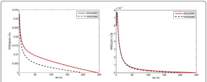
Figure 1Comparison the performance of HRADMM and SRADMM

whereH(·;μ) ={hμ(x1),hμ(x2), . . . ,hμ(xn)}is the half-shrinkage operator [25] defined as

follows:

hμ(xi) =

⎧ ⎨ ⎩

2xi 3 (1 +cos

2

3(π–ϕ(|xi|))), |xi|>

3

√

54 4 μ

2 3,

0, otherwise,

withϕ(x) =arccos(μ₈(xi 3)

–3_2).

For simplicity, we denote algorithms (39) and (40) by SRADMM and HRADMM, respec-tively. The selection of relevant parameters in numerical experiments is given below. We now conduct an experiment to verify convergence of the nonconvex RADMM, and reveal its advantages in sparsity-inducing and efficiency through comparing the performance of HRADMM and SRADMM. In the experiment,m= 511,n= 512, the matrixD∈R511×512 is obtained by unitizing the matrix with randomly generated entries obeying the normal distributionN(0, 1), the noise vectorε∼N(0, 1), the recovery vectorr=Dx0+ε, and the regularization parameters areγ = 0.0015,β= 0.8,α= 2.5.

The experimental results are shown in Fig.1, where the restoration accuracy is measured by means of the mean squared error:

MSEx∗–xk=1 nx

∗_–xk_,

MSEy∗–yk=1 ny

∗_–yk_,

where (x∗,y∗) = (0, 0) is the optimal solution for the problems (37) and (38), respectively. Programming is performed on Matlab R2014a, a computer running the program is con-figured as follows: Windows 7 system, Inter(R) Core(TM) i7-4790 CPU 3.60 GHz, 4 GB memory. Numerical results show that algorithm (7) is efficient and stable. As shown in Fig.1, both sequencesxk_andyk_{were fairly near the true solution. i.e., the convergence is}

justified. It is readily seen that HRADMM converges faster than SRADMM.

5 Conclusion and outlook

Kurdyka–Łojasiewicz property, the strong convergence of the algorithm is analyzed. Fi-nally, the effectiveness of the algorithm is verified by numerical experiments.

Funding

This research was supported by the National Natural Science Foundation of China (Nos. 11601095, 11771383) and by the Natural Science Foundation of Guangxi Province (Nos. 2016GXNSFBA380185, 2016GXNSFDA380019 and

2014GXNSFFA118001).

Availability of data and materials

The authors declare that all data and material in the paper are available and veritable.

Competing interests

The authors declare that they have no competing interests.

Authors’ contributions

All authors contributed equally and significantly in writing this article. All authors wrote, read, and approved the final manuscript.

Authors’ information

JinBao Jian, Ph.D., professor, E-mail: [email protected]; Ye Zhang, E-mail: [email protected]; MianTao Chao, Ph.D., associate professor, E-mail: [email protected].

Author details

1_{College of Mathematics and Information Science, Guangxi University, Nanning, China.}2_{College of Science, Guangxi} University for Nationalities, Nanning, China.

Publisher’s Note

Springer Nature remains neutral with regard to jurisdictional claims in published maps and institutional affiliations.

Received: 11 December 2018 Accepted: 1 July 2019 References

1. Yao, Y.H., Liou, Y.C., Yao, J.C.: Iterative algorithms for the split variational inequality and fixed point problems under nonlinear transformations. J. Nonlinear Sci. Appl.10, 843–854 (2017)

2. Yao, Y.H., Yao, J.C., Liou, Y.C., Postolache, M.: Iterative algorithms for split common fixed points of demicontractive operators without prior knowledge of operator norms. Carpath. J. Math.34, 459–466 (2018)

3. Gabay, D., Mercier, B.: A dual algorithm for the solution of nonlinear variational problems via finite element approximations. Comput. Math. Appl.2(1), 17–40 (1976)

4. He, B.S., Yuan, X.M.: On theO(1/n) convergence rate of the Douglas–Rachford alternating direction method. SIAM J. Numer. Anal.50(2), 700–709 (2012)

5. Monteiro, R.D.C., Svaite, B.F.: Iteration-complexity of block-decomposition algorithms and the alternating direction method of multipliers. SIAM J. Optim.23(1), 475–507 (2013)

6. He, B.S., Yuan, X.M.: On non-ergodic convergence rate of Douglas–Rachford alternating direction method of multipliers. Numer. Math.130(3), 567–577 (2015)

7. Han, D.R., Sun, D.F., Zhang, L.W.: Linear rate convergence of the alternating direction method of multipliers for convex composite quadratic and semi-definite programming. IEEE Trans. Autom. Control60(3), 644–658 (2015)

8. Hong, M.Y.: A distributed, asynchronous, and incremental algorithm for nonconvex optimization: an ADMM approach. IEEE Trans. Control Netw. Syst.5(3), 935–945 (2018)

9. Li, G.Y., Pong, T.K.: Global convergence of splitting methods for nonconvex composite optimization. SIAM J. Optim. 25(4), 2434–2460 (2015)

10. You, S., Peng, Q.Y.: A non-convex alternating direction method of multipliers heuristic for optimal power flow. In: IEEE International Conference on Smart Grid Communications, pp. 788–793. IEEE Press, New York (2014)

11. Hong, M.Y., Luo, Z.Q., Razaviyayn, M.: Convergence analysis of alternating direction method of multipliers for a family of nonconvex problems. SIAM J. Optim.26(1), 3836–3840 (2014)

12. Wang, F.H., Xu, Z.B., Xu, H.K.: Convergence of Bregman alternating direction method with multipliers for nonconvex composite problems (2014). Preprint. Available atarXiv:1410.8625

13. Hong, M., Luo, Z.Q., Razaviyayn, M.: Convergence analysis of alternating direction method of multipliers for a family of nonconvex problems. SIAM J. Optim.26(1), 337–364 (2016)

14. Wang, F.H., Cao, W.F., Xu, Z.B.: Convergence of multi-block Bregman ADMM for nonconvex composite problems. Sci. China Inf. Sci.61(12), 53–64 (2018)

15. Yang, L., Pong, T.K., Chen, X.J.: Alternating direction method of multipliers for a class of nonconvex and nonsmooth problems with applications to background/foreground extraction. SIAM J. Imaging Sci.10(1), 74–110 (2017) 16. Guo, K., Han, D.R., Wu, T.T.: Convergence of alternating direction method for minimizing sum of two nonconvex

functions with linear constraints. Int. J. Comput. Math.94(8), 1–18 (2016)

17. Guo, K., Han, D.R., Wang, Z.W., Wu, T.T.: Convergence of ADMM for multi-block nonconvex separable optimization models. Front. Math. China12(5), 1139–1162 (2017)

18. Zhao, X.P., Ng, K.F., Li, C., Yao, J.C.: Linear regularity and linear convergence of projection-based methods for solving convex feasibility problems. Appl. Math. Optim.78, 613–641 (2018)

20. Mordukhovich, B.S.: Variational Analysis and Generalized Differentiation I: Basic Theory. Springer, Berlin (2006) 21. Attouch, H., Bolte, J., Redont, P., Soubeyran, A.: A proximal alternating minimization and projection methods for

nonconvex problems: an approach based on the Kurdyka–Łojasiewicz inequality. Math. Oper. Res.35(2), 438–457 (2010)

22. Nesterov, Y.: Introduction Lectures on Convex Optimization: A Basic Course. Springer, Berlin (2013)

23. Frankel, P., Garrigos, G., Peypouquet, J.: Splitting methods with variable metric for Kurdyka–Lojasiewicz functions and general convergence rates. J. Optim. Theory Appl.165(3), 874–900 (2015)

24. Daubechies, I., Defrise, M., De Mol, C.: An iterative thresholding algorithm for linear inverse problems with a sparsity constraint. Commun. Pure Appl. Math.57(11), 1413–1457 (2003)

25. Xu, Z., Chang, X., Xu, F., Zhang, H.:l1