Windschitl type approximation formulas for the gamma function

R E S E A R C H

Open Access

Windschitl type approximation formulas

for the gamma function

Zhen-Hang Yang

_{and Jing-Feng Tian}

*_{Correspondence:} [email protected]

1_{College of Science and}

Technology, North China Electric Power University, Baoding, P.R. China Full list of author information is available at the end of the article

Abstract

In this paper, we present four new Windschitl type approximation formulas for the gamma function. By some unique ideas and techniques, we prove that four functions combined with the gamma function and Windschitl type approximation formulas have good properties, such as monotonicity and convexity. These not only yield some new inequalities for the gamma and factorial functions, but also provide a new proof of known inequalities and strengthen known results.

MSC: Primary 41A10; 26A48; secondary 33B10; 26A51

Keywords: Gamma function; Windschitl type approximation formula; Monotonicity; Convexity; Inequality

1 Introduction

Forx> 0, the classical Euler’s gamma functionand psi (digamma) functionψare defined by

(x) = ∞

0

tx–1e–tdt and ψ(x) =

_(x)

(x), (1.1)

respectively. The derivativesψ, ψ, ψ, . . . are known as polygamma functions. The gamma function has various important applications in many branches of science. For this reason, scholars strive to find various better approximations for the factorial or gamma function by using different ideas and techniques, for instance, Ramanujan [1, p. 339], Burn-side [2], Gosper [3], Alzer [4], Shi et al. [5], Batir [6,7], Mortici [8–12], Nemes [13, Corol-lary 4.1], [14], Qi et al. [15,16], Feng and Wang [17], Chen [18–21], Yang et al. [22–25], Lu et al. [26–28], Xu et al. [29]. Some properties of the remainders of certain approximations for the gamma function can be found in [4,16,23,30–35].

In this paper, we are interested in Windschitl’s approximation formula (see [36]) given by

(x+ 1)∼W0(x) =√2πx

x e

x xsinh1

x

x/2

, asx→ ∞. (1.2)

As shown in [21, Eq. (3.18)], the rate of Windschitl’s approximationW0(x) converging to

(x+ 1) is likex–5_{asx→ ∞, and likex}–7_{if one replacesW0(x) with}

W1(x) =√2πx

x e

x xsinh1

x+

1 810x6

x/2

(1.3)

by an easy check. These show thatW0(x) andW1(x) are more accurate approximations for the gamma function. In 2009, Alzer [37] proved that for allx> 0,

√

2πx

x e

x xsinh1

x

x/2

1 + α

x5

<(x+ 1)

<√2πx

x e

x xsinh1

x

x/2

1 + β

x5

(1.4)

with the best possible constantsα= 0 andβ = 1/1620. Recently, Lu, Song and Ma [27] extended Windschitl’s formula to an asymptotic expansion:

(n+ 1)∼√2πn

n e n nsinh 1 n+ a7 n7+

a9 n9 +

a11 n11 +· · ·

n/2

(1.5)

asn→ ∞witha7= 1/810,a9= –67/42525,a11= 19/8505, . . . , and proved that there exists anmsuch that, for everyx>m, the double inequality

xsinh 1 x+ 1 810x7–

67 42525x9

x/2

<√(x+ 1) 2πx(x/e)x <

xsinh 1 x+ 1 810x7

x/2

(1.6)

holds. An explicit formula for determining the coefficients ofn–k(n∈N) was given in [19, Theorem 1] by Chen. Another asymptotic expansion

(x+ 1)∼√2πx

x e

x xsinh1

x

x/2+∞_j=0rjx–j

, asx→ ∞, (1.7)

was presented in the same paper [19, Theorem 2].

Let us consider the four new Windschitl type approximation formulas, asx→ ∞, which are

(x+ 1)∼√2πx

x e

x xsinh1

x

x/2

exp

1 1620x5

:=W01(x), (1.8)

(x+ 1)∼√2πx

x e

x xsinh1

x

x/2

exp

1 1620x5 –

11 18,900x7

:=W02(x), (1.9)

(x+ 1)∼√2πx

x e

x xsinh1

x

x/2

1 + 1 1620x5

:=W₀₁∗(x), (1.10)

(x+ 1)∼√2πx

x e

x xsinh1

x

x/2

1 + 1 1620x5 –

11 18,900x7

=W₀₂∗(x). (1.11)

The aim of this paper is, by investigating the monotonicity and convexity of the functions

to establish some new sharp inequalities between the gamma function(x+ 1) and Winds-chitl’s approximation formulaW0(x). As a by-product, a concise proof of Alzer inequalities

(1.4) is presented, and a strengthening for Lu et al.’s inequalities (1.6) is given.

The rest of this paper is organized as follows. In Sect.2, three lemmas are given, which are crucial to the proofs of our results. In Sect. 3, five monotonicity and convexity re-sults for the functions constructed from the gamma function and Windschilt’s formula are proved. Some new inequalities between the gamma or factorial functions with Wind-schilt’s formula are established in Sect.4. In Sect.5, numeric comparisons of several better approximation formulas are presented.

2 Lemmas

To prove our results, we need three lemmas as follows.

Lemma 1 The inequalities

x x

2₊71 84 x4₊13

14x2+ 27 560

<ψ

x+1 2

, (2.1)

x x

4₊227 66x2+

4237 2640 x6₊155

44x4+ 329 176x2+

375 4928

<ψ

x+1 2

<1

x x4₊67

36x2+ 256 945 x4₊35

18x2+ 407 1008

(2.2)

hold for x> 0.

Proof The inequality (2.1) was proved in [38, Remark 2.2]. Let

g1(x) =ψ

x+1 2

–1

x x4₊67

36x2+ 256 945 x4₊35

18x2+ 407 1008

,

g2(x) =ψ

x+1 2

–x x 4₊227

66x2+ 4237 2640 x6₊155

44x4+ 329 176x2+

375 4928

.

Then we have

g1(x+ 1) –g1(x) =ψ

x+3 2

– 1

x+ 1

(x+ 1)4+67₃₆(x+ 1)2+256₉₄₅ (x+ 1)4₊35

18(x+ 1)2+ 407 1008

–ψ

x+1 2

+1

x x4₊67

36x2+ 256 945 x4₊35

18x2+ 407 1008

= 921,600×x(2x+ 1)2(x+ 1) 1008x4+ 1960x2+ 407–1

× 1008x4+ 4032x3+ 8008x2+ 7952x+ 3375–1> 0.

Hence, we conclude that

g1(x) <g1(x+ 1) <· · ·< lim

n→∞g1(x+n) = 0,

Analogously, we have

g2(x+ 1) –g2(x)

=ψ

x+3 2

– (x+ 1)((x+ 1)

4₊227 66(x+ 1)

2₊4237 2640)

(x+ 1)6₊155

44(x+ 1)4+ 329

176(x+ 1)2+ 375 4928

–ψ

x+1 2

+ x(x

4₊227 66x

2₊4237 2640) x6₊155

44x4+ 329 176x2+

375 4928

= –58,982,400×(2x+ 1)2 4928x6+ 17,360x4+ 9212x2+ 375–1

× 4928x6+ 29,568x5+ 91,280x4+ 168,000x3

+ 187,292x2+ 117,432x+ 31,875–1

< 0.

It then follows that

g2(x) >g2(x+ 1) >· · ·> lim

n→∞g2(x+n) = 0,

which proves the second formula of (2.2). This completes the proof.

Lemma 2 The inequalities

t2

sinh2t > 1 –

1 3t

2₊ 1

15t

4_– 2

189t

6_{, (2.3)}

t2

sinh2t > 1 –

1 3t

2₊ 1

15t

4_– 2

189t

6₊ 1

675t

8_– 2

10,395t

10 _(2.4)

hold for all t> 0.

Proof The inequalities in question are equivalent to

h1(t) =

2 189t

6_– 1

15t

4₊1

3t

2_{– 1}

cosh2t– 1 2t2 + 1 > 0

and

h2(t) =

2 10,395t

10_– 1

675t

8₊ 2

189t

6_– 1

15t

4₊1

3t

2_{– 1}

cosh2t– 1 2t2 + 1 > 0

fort> 0, respectively.

Expanding into a power series yields

h1(t) =

2 189t

6_– 1

15t

4₊1

3t

2_{– 1}

∞

n=0

22n+1 (2n+ 2)!t

2n_{+ 1}

= 2 189

∞

n=3

(2t)2n

32(2n– 4)!– 1 15

∞

n=2

(2t)2n

8(2n– 2)!+ 1 3

∞

n=1

(2t)2n

– 2

∞

n=0

(2t)2n (2n+ 2)!+ 1 :=

1 1890

∞

n=3

(n– 3)×p5(n) (2n+ 2)! (2t)

2n_,

where

p5(n) = 40n5+ 60n4– 122n3– 543n2– 296n+ 1050.

We assert thatp5(n) > 0 forn≥3, sincep5(n) can be written as

p5(n) = 40(n– 3)5+ 660(n– 3)4+ 4198(n– 3)3+ 12,399(n– 3)2+ 15,832(n– 3) + 6561,

which is evidently positive forn≥3. Henceh1(t) > 0 for allt> 0. While

h2(t) =h1(t) +

2 10,395t

10_– 1

675t

8

∞

n=0

22n+1 (2n+ 2)!t

2n

= 1 1890

∞

n=3

(n– 3)×p5(n) (2n+ 2)! (2t)

2n₊ 2

10,395

∞

n=5

(2t)2n

29_{(2n– 8)!}

– 1 675

∞

n=4

(2t)2n 27_{(2n– 6)!} :=

1 415,800

∞

n=5

(n– 5)×p9(n) (2n+ 2)! (2t)

2n_,

where

p9(n) = 160n9– 1200n8+ 2368n7– 1768n6+ 2354n5+ 14,845n4

– 6403n3– 70,782n2– 57,384n+ 138,600.

It is easy to check that

p9(n) = 160m9+ 6000m8+ 98,368m7+ 921,112m6+ 5392,514m5+ 20,270,695m4

+ 48,258,997m3+ 68,827,423m2+ 51,883,321m+ 15,041,130 > 0,

form=n– 5≥0, which provesh2(t) > 0 fort> 0. The proof is complete.

The following lemma offers a simple criterion to determine the sign of a class of special polynomials on given interval contained in (0,∞) without using Descartes’ Rule of Signs, which plays an important role in studying certain special functions, see, for example, [39, 40]. A series version can be found in [41,42].

Lemma 3([39, Lemma 7]) Let n∈Nand m∈N∪ {0}with n>m and let Pn(t)be an nth degree polynomial defined by

Pn(t) =

n

i=m+1 aiti–

m

i=0

aiti, (2.5)

Consequently,for a given t0> 0,if Pn(t0) > 0then Pn(t) > 0for t∈(t0,∞)and if Pn(t0) < 0

then Pn(t) < 0for t∈(0,t0).

3 Monotonicity and convexity

Theorem 1 T he function

f0(x) =ln(x+ 1) –ln

√

2π–

x+1 2

lnx+x–x 2ln

xsinh1

x

is strictly decreasing and convex on(0,∞).

Proof Differentiation yields

f₀(x) =ψ(x+ 1) –1 2ln

xsinh1

x

+ 1

2xcoth

1

x–lnx–

1 2x–

1 2,

f₀(x) =ψ(x+ 1) + 1 2x3

1

sinh2(1/x)– 3 2x+

1 2x2.

Replacingxby (x+ 1/2) in inequality (2.1) leads to

ψ(x+ 1) >5 6

(2x+ 1)(21x2_{+ 21x+ 23)}

35x4_{+ 70x}3_{+ 85x}2_{+ 50x+ 12},

and using which tof₀(x) gives

f₀(x) >5 6

(2x+ 1)(21x2+ 21x+ 23) 35x4_{+ 70x}3_{+ 85x}2_{+ 50x+ 12}

+ 1 2x3

1

sinh2(1/x)– 3 2x+

1 2x2 =f01

1

x

.

Simplifying yields

f01(t) =

1 2

t3

sinh2t+

1 6

t(36t5_{+ 42t}4_{– 80t}3_{– 220t}2_{– 210t– 105)}

12t4_{+ 50t}3_{+ 85t}2_{+ 70t+ 35}

= t 12

f02(t)

(12t4_{+ 50t}3_{+ 85t}2_{+ 70t+ 35)sinh}2_t,

where

f02(t) = 36t5+ 42t4– 80t3– 220t2– 210t– 105

cosh2t

+ 72t6+ 264t5+ 468t4+ 500t3+ 430t2+ 210t+ 105.

Expanding into a power series gives

f02(t) =

36

∞

n=2

22n–4

(2n– 4)!t

2n+1_{– 80}

∞

n=1

22n–2

(2n– 2)!t

2n+1_{– 210}

∞

n=0

22n

(2n)!t

2n+1

+

42

∞

n=2

22n–4

(2n– 4)!t

2n_{– 220}

∞

n=1

22n–2

(2n– 2)!t

2n_{– 105}

∞

n=0

22n

(2n)!t

2n

=

∞

n=4

(n– 3)(36n3+ 19n+ 70)22n (2n)! t

2n+1

+

∞

n=4

(84n4_{– 252n}3_{– 209n}2_{+ 157n– 210)2}2n–2

(2n)! t

2n_{> 0,}

where the inequality holds due to

84n4– 252n3– 209n2+ 157n– 210

= 84(n– 4)4+ 1092(n– 4)3+ 4831(n– 4)2+ 7893(n– 4) + 2450 > 0

forn≥4.

It then follows that f01(t) > 0 for t > 0, so f₀(x) > 0 for x > 0. This yields f₀(x) <

limx→∞f0(x) = 0, which proves the desired result.

Theorem 2 The function

f₁∗(x) =ln(x+ 1) –ln√2π–

x+1 2

lnx+x–x 2ln

xsinh1

x

–ln

1 + 1

1620x5

is strictly increasing and concave on(0,∞).

Proof Differentiation yields

f₁∗(x) =ψ(x+ 1) –1 2ln

xsinh1

x

+ 1

2xcoth

1

x

–lnx– 1 2x–

1 2+

5

x(1620x5_{+ 1)},

f₁∗(x) =ψ(x+ 1) + 1 2x3

1

sinh2(1/x)– 3 2x+

1 2x2 – 5

9720x5+ 1

x2_(1620x5_{+ 1)}2.

Sincelimx→∞f1∗(x) = 0, it suffices to provef1∗(x) < 0 forx> 0. Replacingxby (x+ 1/2) in

the right-hand side inequality of (2.2) leads to

ψ(x+ 1) < 1 30

3780x4_{+ 7560x}3_{+ 12,705x}2_{+ 8925x+ 3019}

(2x+ 1)(63x4_{+ 126x}3_{+ 217x}2_{+ 154x+ 60)}, (3.1)

which indicates that

f₁∗(x) < 1 30

3780x4_{+ 7560x}3_{+ 12,705x}2_{+ 8925x+ 3019}

(2x+ 1)(63x4_{+ 126x}3_{+ 217x}2_{+ 154x+ 60)}

+ 1 2x3

1

sinh2(1/x)– 3 2x+

1 2x2 – 5

9720x5_{+ 1} x2_(1620x5_{+ 1)}2 :=f

∗

11

1

x

,

where

f₁₁∗(t) = t

3

cosh2t– 1– 3 2t+

1 2t

2_{– 5t}7 t5+ 9720

(t5_{+ 1620)}2

+ 1 30

t(3019t4_{+ 8925t}3_{+ 12,705t}2_{+ 7560t+ 3780)}

Using the inequality

cosh2t– 1 >

4

n=1

22n (2n)!t

2n_{= 2t}2₊2

3t

4₊ 4

45t

6₊ 2

315t

8

yields

f₁₁∗(t)

< t

3

2t2₊2 3t4+

4 45t6+

2 315t8

–3 2t+

1 2t

2_{– 5t}7 t5+ 9720

(t5_{+ 1620)}2

+ 1 30

t(3019t4_{+ 8925t}3_{+ 12,705t}2_{+ 7560t+ 3780)}

(t+ 2)(60t4_{+ 154t}3_{+ 217t}2_{+ 126t+ 63)}

= –1 30

× t9×f12∗(t)

(t5_{+ 1620)}2_{(t+ 2)(t}6_{+ 14t}4_{+ 105t}2_{+ 315)(60t}4_{+ 154t}3_{+ 217t}2_{+ 126t+ 63)}

< 0

fort> 0, where the inequality holds due to

f₁₂∗(t) = 8100t14+ 39,690t13+ 193,586t12+ 645,960t11+ 2,028,124t10

+ 90,019,275t9+ 406,666,800t8+ 1976,029,740t7+ 6395,589,900t6

+ 20,173,546,260t5+ 51,035,406,750t4+ 110,592,337,500t3

+ 184,843,490,400t2+ 254,068,164,000t+ 101,627,265,600 > 0

fort> 0. This implies thatf₂(x) < 0 for allx> 0, and the proof is complete.

Theorem 3 The function

f1(x) =ln(x+ 1) –ln√2π–

x+1 2

lnx+x–x 2ln

xsinh1

x

– 1

1620x5

is strictly increasing and concave on(0,∞).

Proof We clearly see that

f1(x) =f₁∗(x) +D

1 1620x5

,

whereD(y) =ln(1 +y) –y. By Theorem2,f₁∗is strictly increasing and concave on (0,∞), so if we provex→D(y) is strictly increasing and concave on (0,∞), then so will bef1, and the proof will be complete. Now we easily check that forx> 0,

dD(y)

dx =

1

d2_D(y) dx2 = –

1 54

2970x5_{+ 1} x7_(1620x5_{+ 1)}2 < 0,

which completes the proof.

Theorem 4 The function

f2(x) =ln(x+ 1) –ln√2π–

x+1 2

lnx+x

–x 2ln

xsinh1

x

– 1

1620x5 +

11 18,900x7

is strictly decreasing and convex on(0,∞).

Proof Differentiation yields

f₂(x) =ψ(x+ 1) –1 2ln

xsinh1

x

+ 1

2xcoth

1

x

–lnx– 1 2x–

1 2+

1 324x6 –

11 2700x8,

f₂(x) =ψ(x+ 1) + 1 2x3

1

sinh2(1/x)– 3 2x+

1 2x2–

1 54x7+

22 675x9.

Sincelim_x→∞f₂(x) = 0, it suffices to provef₂(x) > 0 forx> 0. Replacingxby (x+ 1/2) in the left-hand side inequality of (2.2) leads to

ψ(x+ 1) > 7 30

(2x+ 1)(165x4_{+ 330x}3_{+ 815x}2_{+ 650x+ 417)}

77x6_{+ 231x}5_{+ 560x}4_{+ 735x}3_{+ 623x}2_{+ 294x+ 60},

and applying which tof₂(x) gives

f₂(x) > 7 30

(2x+ 1)(165x4+ 330x3+ 815x2+ 650x+ 417) 77x6_{+ 231x}5_{+ 560x}4_{+ 735x}3_{+ 623x}2_{+ 294x+ 60}

+ 1 2x3

1

sinh2(1/x)– 3 2x+

1 2x2 –

1 54x7+

22 675x9 =f21

1

x

.

Making a change of variablet= 1/xyields

f21(t) = 7 30

t(t+ 2)(417t4+ 650t3+ 815t2+ 330t+ 165) 60t6_{+ 294t}5_{+ 623t}4_{+ 735t}3_{+ 560t}2_{+ 231t+ 77}

–3 2t+

1 2t

2_– 1

54t

7₊ 22

675t

9₊t

2

t2

sinh2t.

We distinguish two cases to provef21(t) > 0 for allt> 0. Case1:t≥1. Application of inequality (2.3) gives

f21(t) >

7 30

t(t+ 2)(417t4_{+ 650t}3_{+ 815t}2_{+ 330t+ 165)}

60t6_{+ 294t}5_{+ 623t}4_{+ 735t}3_{+ 560t}2_{+ 231t+ 77}–

3 2t+

1 2t

2

– 1 54t

7₊ 22

675t

9₊t

2

1 –1 3t

2₊ 1

15t

4_– 2

189t

6

= 1 9450

t9_×p6(t)

60t6_{+ 294t}5_{+ 623t}4_{+ 735t}3_{+ 560t}2_{+ 231t+ 77},

where

p6(t) = 18,480t6+ 90,552t5+ 178,384t4+ 160,230t3+ 51,205t2– 1617t– 539.

Clearly,p6(t) > 0 fort≥1, sof21(t) > 0 fort≥1.

Case2: 0 <t< 1. Using inequality (2.4) yields

f21(t) >

7 30

t(t+ 2)(417t4_{+ 650t}3_{+ 815t}2_{+ 330t+ 165)}

60t6_{+ 294t}5_{+ 623t}4_{+ 735t}3_{+ 560t}2_{+ 231t+ 77}–

3 2t+

1 2t

2

– 1 54t

7₊ 22

675t

9₊t

2

1 –1 3t

2₊ 1

15t

4_– 2

189t

6₊ 1

675t

8_– 2

10,395t

10

= t

11_×q 6(t)

60t6_{+ 294t}5_{+ 623t}4_{+ 735t}3_{+ 560t}2_{+ 231t+ 77},

where

q6(t) = – 4 693t

6_– 14

495t

5₊2881

1485t

4₊4816

495t

3₊400,919

20,790 t

2₊1573

90 t+ 1573

270 .

Since the coefficients of polynomialq6(t) satisfy the conditions of Lemma3andq6(1) = 53,681/990 > 0, we find thatq6(t) > 0 fort∈(0, 1), and thenf21(t) > 0 fort∈(0, 1).

This ends the proof.

Theorem 5 The function

f₂∗(x) =ln(x+ 1) –ln√2π–

x+1 2

lnx+x

–x 2ln

xsinh1

x

–ln

1 + 1

1620x5 –

11 18,900x7

is strictly decreasing and convex on[4/3,∞).

Proof We easily see that

f₂∗(x) =f2(x) –D

1 1620x5 –

11 18,900x7

,

whereD(y) =ln(1 +y) –y. By Theorem4,f2is strictly decreasing and convex on (0,∞), so if we provex→D(y) is strictly increasing and concave on [4/3,∞), then so will bef₂∗, and the proof will be complete. Now we easily check that forx≥4/3,

dD(y)

dx =

1 8100

(25x2– 33)(35x2– 33)

x8_(35x2_{+ 56,700x}7_{– 33)}> 0,

d2_D(y) dx2 = –

p11(x)

where the last inequality holds due to

p11(x) = 67,375x11– 180,180x9+ 114,345x7+

1225 54 x

6_–2233

27 x

4₊8591

90 x

2_–2662

75

= 385x7

175

x2–16 9

2

+1388 9

x2–16 9

+1465

81

+ 1 1350x

2 _175x2_{– 319}2

+242 675

56

x2–16 9

+5

9

> 0,

which completes the proof.

4 Inequalities

As is well known, analytic inequalities [43–45] play a very important role in different branches of modern mathematics. Using the theorems presented in the previous section, we can obtain some new inequalities for the gamma function and factorial function related to Windschitl’s formula.

Corollary 1 Let W0(x)be defined by(1.2).Then the inequalities

max

1,exp

1 1620x5 –

11 18,900x7

<(x+ 1)

W0(x) < 1 + 1

1620x5 <exp

1 1620x5

(4.1)

hold for all x> 0.If x≥√33/35,then we have

1 + 1 1620x5 –

11

18,900x7 <exp

1 1620x5 –

11 18,900x7

<(x+ 1)

W0(x) < 1 + 1

1620x5 <exp

1 1620x5

. (4.2)

Proof The first and second inequalities in (4.1) follow directly from the monotonicity of

f0,f2andf₁∗on (0,∞) given in Theorems1,4and2, respectively, due tof0(∞) =f2(∞) =

f1∗(∞) = 0. The third one holds due to a simple inequality 1 +y<eyfory> 0. The proof of

inequalities (4.2) is similar, which completes the proof.

Using the monotonicity off0,f1∗andf2on (0,∞) and noting that

f0(1) =ln√ e

2πsinh1, f

∗

1(1) =ln

1620 1621

e

√

2πsinh1

, f2(1) =lne

28,349/28,350

√

2πsinh1,

we immediately get the following corollary.

Corollary 2 For n∈N,the inequalities

1 <√ n! 2πn(n

e)n(nsinh 1 n)n/2

≤α0,

β₁∗

1 + 1

1620n5

≤√ n!

2πn(n

e)n(nsinh 1 n)n/2

exp

1 1620n5 –

11 18,900n7

<√ n! 2πn(n_e)n_(nsinh1

n)n/2

≤α2exp

1 1620n5–

11 18,900n7

hold with the best constantsα0=e/

√

2πsinh1≈1.000,34,β₁∗= 1620e/(1621√2πsinh1)≈ 0.999,72andα2=e28,349/28,350/

√

2πsinh1≈1.000,30.

The proof of inequalities (1.4) presented by Alzer [37] seems to be somewhat compli-cated. With the aid of the first and second inequalities in (4.1), we can give a new and simpler proof.

Proof of inequalities(1.4) The sufficiency for the inequalities (1.4) to hold forx> 0 follows by the first and second inequalities in (4.1). The necessary condition for the left-hand side inequality of (1.4) to hold forx> 0 follows from the following relation:

lim

x→0+

ln(x+ 1) –ln√2π– (x+1

2)lnx+x– x

2ln(xsinh 1

x) –ln(1 + α x5)

ln(1/x)

= ⎧ ⎨ ⎩

1

2 ifα= 0,

–9₂ ifα= 0.

While the necessary condition for the right-hand side of (1.4) to hold forx> 0 follows from the limit relation

lim

x→∞

ln(x+ 1) –ln√2π– (x+1

2)lnx+x– x

2ln(xsinh 1

x) –ln(1 + β x5) x–5

= 1

1620–β≤0.

This completes the proof.

The following corollary offers a strengthening for Lu et al.’s inequalities (1.6).

Corollary 3 The inequalities

xsinh

1

x+

1 810x7–

67 42,525x9

x/2

<

xsinh1

x

x/2

exp

1 1620x5 –

11 18,900x7

<√(x+ 1) 2πx(x/e)x

<

xsinh1

x

x/2

exp

1 1620x5

<

xsinh

1

x+

1 810x7

x/2

(4.3)

hold for x>c, where c= 0for the second,third and fourth inequalities, while c=x0≈

0.43738for the first one,here x0is the unique solution of the equation

1

x+

1 810x7 –

67 42,525x9= 0

Proof Clearly, the second and third inequalities of (4.3) follow by the first and second inequalities in (4.1). It remains to prove the first and last inequalities of (4.3).

(i) The last one is equivalent to

x

2ln

xsinh

1

x+

1 810x7

>x

2ln

xsinh1

x

+ 1

1620x5,

or equivalently,

h3(t) =ln sinh

t+ 1 810t

7

–ln sinht– 1 810t

6_{> 0}

fort= 1/x> 0. Denote byl(t) =ln sinhtandt2= (t+t7_{/810). Then by Taylor formula we}

have

h3(t) =l(t2) –l(t) – 1 810t

6_{= (t2–t)l(t) +}l(t)

2! (t2–t)

2₊l(ξ)

3! (t2–t)

3_– 1

810t

6_,

wheret<ξ<t+t7/810. Sincel(t) = 2(cosht)/sinh3t> 0, we get

h3(t) > 1 810t

7cosht

sinht – t14

2×8102

1

sinh2t–

1 810t

6_:= t6×h31(t)

2×8102_sinh2_t,

where

h31(t) = 810tsinh2t– 810cosh2t+ 810 –t8.

Due to

h31(t) = 540t4+ 144t6+

101 7 t

8_{+ 810}

∞

n=5

(n– 1)22n

(2n)! t

2n_{> 0,}

we conclude thath3(t) > 0 fort> 0.

(ii) To ensure that the first inequality holds, it is necessary to establish

xsinh

1

x+

1 810x7–

67 42,525x9

> 0

forx> 0, for which it suffices so show that

1

x+

1 810x7 –

67 42,525x9=

85,050x8_{+ 105x}2_{– 134}

85,050x9 > 0.

By Lemma3, the numerator in the above fraction, as an 8th degree polynomial, has a unique zerox0on (0,∞). Numeric computation givesx0≈0.437,38.

Now the first inequality is equivalent to

x

2ln

xsinh

1

x+

1 810x7 –

67 42,525x9

<x

2ln

xsinh1

x

+ 1

1620x5 –

or equivalently,

h4(t) =ln

sinh

t+ 1 810t

7_– 67

42,525t

9

–ln(sinht) – 1 810t

6₊ 11

9450t

8_{< 0}

fort= 1/x∈(0, 1/x0), where 1/x0≈2.28632 is clearly the unique zero of the polynomial

t1≡t1(t) =t+

1 810t

7_– 67

42,525t

9

on (0,∞). In view ofl(t) = –1/sinh2t< 0, we have

h4(t) =l(t1) –l(t) –

1 810t

6₊ 11

9450t

8_{< (t}

1–t)l(t) –

1 810t

6₊ 11

9450t

8

=

1 810t

7_– 67

42,525t

9

cosht

sinht –

1 810t

6₊ 11

9450t

8

= – 1 85,050

t6

sinht 105sinht– 105tcosht+ 134t

3_{cosht– 99t}2_sinht

= – 1 85,050

t6

sinht

∞

n=3

4(268n– 99)(n– 1)(n– 2) (2n– 1)! t

2n–1_{< 0,}

which completes the proof.

Remark1 Clearly, the proof of Corollary3can also be regarded as a new proof of Lu et al.’s inequalities (1.6). Moreover, our proof gives the minimum value ofm, i.e.,min(m) =

x0≈0.437,38, such that the the double inequality (1.6) holds for allx>x0.

5 Numeric comparisons

By the asymptotic expansion listed in [46, Eq. (6.1.40)]

ln(x+ 1)∼ln√2π+

x+1 2

lnx–x+

∞

n=1

B2n

2n(2n– 1)x2n–1, (5.1)

we easily verify that our four approximation formulasW01(x),W₀₁∗(x),W02(x) andW₀₂∗(x), defined by (1.8), (1.10), (1.9) and (1.11), respectively, have the following limit relations:

lim

x→∞

ln(x+ 1) –lnW01(x)

x–7 =_xlim_→∞

ln(x+ 1) –lnW01∗(x)

x–7 = –

198 340,200,

lim

x→∞

ln(x+ 1) –lnW02(x)

x–9 =_xlim_→∞

ln(x+ 1) –lnW₀₂∗(x)

x–9 =

143 170,100.

Also, for another approximation formulaW1(x) defined by (1.3), we have

lim

x→∞

ln(x+ 1) –lnW1(x)

x–7 = –

163 340,200.

Denote the two approximation formulas generated by the double inequality (1.6) by

WL1(x) =

√

2πx

x e

x xsinh

1

x+

1 810x7

x/2

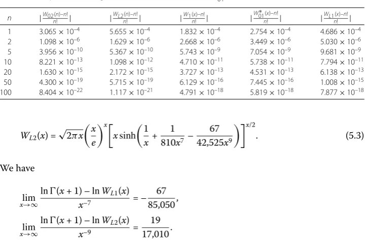
Table 1 Comparison amongW02(1.9),WL2(5.3),W1(1.3),W∗01(1.10) andWL1(5.2)

n |W02(n)–n!

n! | |WL2(

n)–n!

n! | |

W₁₍x)–n!

n! | |

W₀₁∗(x)–n!

n! | |WL1(

x)–n!

n! |

1 3.065×10–4 _5.655×10–4 _1.832×10–4 _2.754×10–4 _4.686×10–4

2 1.098×10–6 _1.629×10–6 _2.668×10–6 _3.449×10–6 _5.030×10–6

5 3.956×10–10 _5.367×10–10 _5.743×10–9 _7.054×10–9 _9.681×10–9

10 8.221×10–13 _1.098×10–12 _4.710×10–11 _5.738×10–11 _7.794×10–11

20 1.630×10–15 _2.172×10–15 _3.727×10–13 _4.531×10–13 _6.138×10–13

50 4.300×10–19 _5.715×10–19 _6.129×10–16 _7.445×10–16 _1.008×10–15

100 8.404×10–22 _1.117×10–21 _4.791×10–18 _5.819×10–18 _7.877×10–18

WL2(x) =√2πx

x e

x xsinh

1

x+

1 810x7–

67 42,525x9

x/2

. (5.3)

We have

lim

x→∞

ln(x+ 1) –lnWL1(x)

x–7 = –

67 85,050,

lim

x→∞

ln(x+ 1) –lnWL2(x)

x–9 =

19 17,010.

These, in combination with Corollaries2,1and3, show that the approximation for-mulaW02(x) given by (1.9) is the best among those listed above, which can be seen from comparison Table1.

6 Conclusion

In this paper, we provide four Windschitl type approximation formulas for the gamma function, and prove that those functions, involving the gamma function and Windschitl type functions, have good properties, including monotonicity and convexity. From these facts we obtain some new sharp Windschitl type bounds for the gamma and factorial functions. These sharp inequalities, together with numerical comparisons, illustrate that

W02(x) defined by (1.9) is the best approximation formula among those mentioned in Sect.5.

Moreover, we give a simple proof of Alzer’s inequalities (1.4), and improve and strengthen Lu et al.’s inequalities (1.6).

It is worth mentioning that our proofs of Theorems1–5are subtle and interesting, since the approximations deal with the gamma and hyperbolic sine functions, and it is difficult to establish their monotonicity and convexity by usual methods. Evidently, Lemmas2and 3play important roles.

Acknowledgements

The authors would like to express their sincere thanks to the anonymous referees for their great efforts to improve this paper.

Funding

This work was supported by the Fundamental Research Funds for the Central Universities (No. 2015ZD29) and the Higher School Science Research Funds of Hebei Province of China (No. Z2015137).

Competing interests

The authors declare that they have no competing interests.

Authors’ contributions

Author details

1_{College of Science and Technology, North China Electric Power University, Baoding, P.R. China.}2_{Department of Science}

and Technology, State Grid Zhejiang Electric Power Company Research Institute, Hangzhou, P.R. China.

Publisher’s Note

Springer Nature remains neutral with regard to jurisdictional claims in published maps and institutional affiliations.

Received: 3 March 2018 Accepted: 30 September 2018

References

1. Ramanujan, S.: The Lost Notebook and Other Unpublished Papers. Springer, Berlin (1988) 2. Burnside, W.: A rapidly convergent series for logN!. Messenger Math.46, 157–159 (1917)

3. Gosper, R.W.: Decision procedure for indefinite hypergeometric summation. Proc. Natl. Acad. Sci. USA75, 40–42 (1978).https://doi.org/10.1073/pnas.75.1.40

4. Alzer, H.: On some inequalities for the gamma and psi functions. Math. Comput.66(217), 373–389 (1997).

https://doi.org/10.1090/S0025-5718-97-00807-7

5. Shi, X., Liu, F., Hu, M.: A new asymptotic series for the Gamma function. J. Comput. Appl. Math.195, 134–154 (2006).

https://doi.org/10.1016/j.cam.2005.03.081

6. Batir, N.: Inequalities for the gamma function. Arch. Math.91, 554–563 (2008).

https://doi.org/10.1007/s00013-008-2856-9

7. Batir, N.: Bounds for the Gamma function. Results Math.72, 865–874 (2017).

https://doi.org/10.1007/s00025-017-0698-0

8. Mortici, C.: A new Stirling series as continued fraction. Numer. Algorithms56(1), 17–26 (2011).

https://doi.org/10.1007/s11075-010-9370-4

9. Mortici, C.: Improved asymptotic formulas for the gamma function. Comput. Math. Appl.61, 3364–3369 (2011).

https://doi.org/10.1016/j.camwa.2011.04.036

10. Mortici, C.: Further improvements of some double inequalities for bounding the gamma function. Math. Comput. Model.57, 1360–1363 (2013).https://doi.org/10.1016/j.mcm.2012.11.020

11. Mortici, C.: A continued fraction approximation of the gamma function. J. Math. Anal. Appl.402, 405–410 (2013).

https://doi.org/10.1016/j.jmaa.2012.11.023

12. Mortici, C.: A new fast asymptotic series for the gamma function. Ramanujan J.38, 549–559 (2015).

https://doi.org/10.1007/s11139-014-9589-0

13. Nemes, G.: New asymptotic expansion for the Gamma function. Arch. Math. (Basel)95, 161–169 (2010).

https://doi.org/10.1007/s00013-010-0146-9

14. Nemes, G.: More accurate approximations for the gamma function. Thai J. Math.9(1), 21–28 (2011)

15. Guo, B.N., Zhang, Y.J., Qi, F.: Refinements and sharpenings of some double inequalities for bounding the gamma function. J. Inequal. Pure Appl. Math.9(1), Article ID 17 (2008)

16. Qi, F.: Integral representations and complete monotonicity related to the remainder of Burnside’s formula for the gamma function. J. Comput. Appl. Math.268, 155–167 (2014).https://doi.org/10.1016/j.cam.2014.03.004

17. Feng, L., Wang, W.: Two families of approximations for the gamma function. Numer. Algorithms64, 403–416 (2013).

https://doi.org/10.1007/s11075-012-9671-x

18. Chen, C.-P.: Unified treatment of several asymptotic formulas for the gamma function. Numer. Algorithms64, 311–319 (2013).https://doi.org/10.1007/s11075-012-9667-6

19. Chen, C.-P.: Asymptotic expansions of the gamma function related to Windschitl’s formula. Appl. Math. Comput.245, 174–180 (2014).https://doi.org/10.1016/j.amc.2014.07.080

20. Chen, C.-P., Paris, R.B.: Inequalities, asymptotic expansions and completely monotonic functions related to the gamma function. Appl. Math. Comput.250, 514–529 (2015).https://doi.org/10.1016/j.amc.2014.11.010

21. Chen, C.-P.: A more accurate approximation for the gamma function. J. Number Theory164, 417–428 (2016).

https://doi.org/10.1016/j.jnt.2015.11.007

22. Yang, Z.-H., Chu, Y.-M.: Asymptotic formulas for gamma function with applications. Appl. Math. Comput.270, 665–680 (2015).https://doi.org/10.1016/j.amc.2015.08.087

23. Yang, Z.-H.: Approximations for certain hyperbolic functions by partial sums of their Taylor series and completely monotonic functions related to gamma function. J. Math. Anal. Appl.441, 549–564 (2016).

https://doi.org/10.1016/j.jmaa.2016.04.029

24. Yang, Z.-H., Tian, J.-F.: Monotonicity and inequalities for the gamma function. J. Inequal. Appl.2017, Article ID 317 (2017).https://doi.org/10.1186/s13660-017-1591-9

25. Yang, Z.-H., Tian, J.-F.: An accurate approximation formula for gamma function. J. Inequal. Appl.2018, Article ID 56 (2018).https://doi.org/10.1186/s13660-018-1646-6

26. Lu, D.: A new sharp approximation for the Gamma function related to Burnside’s formula. Ramanujan J.35(1), 121–129 (2014).https://doi.org/10.1007/s11139-013-9534-7

27. Lu, D., Song, L., Ma, C.: A generated approximation of the gamma function related to Windschitl’s formula. J. Number Theory140, 215–225 (2014).https://doi.org/10.1016/j.jnt.2014.01.023

28. Lu, D., Song, L., Ma, C.: Some new asymptotic approximations of the gamma function based on Nemes’ formula, Ramanujan’s formula and Burnside’s formula. Appl. Math. Comput.253, 1–7 (2015).

https://doi.org/10.1016/j.amc.2014.12.077

29. Xu, A., Hu, Y., Tang, P.: Asymptotic expansions for the gamma function. J. Number Theory169, 134–143 (2016).

https://doi.org/10.1016/j.jnt.2016.05.020

30. Qi, F., Niu, D.-W., Guo, B.-N.: Monotonic properties of differences for remainders of psi function. Int. J. Pure Appl. Math. Sci.4(1), 59–66 (2007)

32. Shi, X.-Q., Liu, F.-S., Qu, H.-M.: The Burnside approximation of gamma function. Anal. Appl.8(3), 315–322 (2010).

https://doi.org/10.1142/S0219530510001643

33. Qi, F., Guo, B.-N.: Some properties of extended remainder of Binet’s first formula for logarithm of gamma function. Math. Slovaca60(4), 461–470 (2010).https://doi.org/10.2478/s12175-010-0025-7

34. Qi, F., Guo, B.-N.: Integral representations and complete monotonicity of remainders of the Binet and Stirling formulas for the gamma function. Rev. R. Acad. Cienc. Exactas Fís. Nat., Ser. A Mat.111(2), 425–434 (2017).

https://doi.org/10.1007/s13398-016-0302-6

35. Yang, Z.-H., Tian, J.-F.: Two asymptotic expansions for gamma function related to Windschitl’s formula. Open Math.16, 1048–1060 (2018).https://doi.org/10.1515/math-2018-0088

36. Smith, W.D.: The gamma function revisited.http://schule.bayernport.com/gamma/gamma05.pdf(2006) 37. Alzer, H.: Sharp upper and lower bounds for the gamma function. Proc. R. Soc. Edinb.139A, 709–718 (2009).

https://doi.org/10.1017/S0308210508000644

38. Yang, Z.-H., Chu, Y.-M., Zhang, X.-H.: Sharp bounds for psi function. Appl. Math. Comput.268, 1055–1063 (2015).

https://doi.org/10.1016/j.amc.2015.07.012

39. Yang, Z.-H., Chu, Y.-M., Tao, X.-J.: A double inequality for the trigamma function and its applications. Abstr. Appl. Anal.

2014, Article ID 702718 (2014).https://doi.org/10.1155/2014/702718

40. Yang, Z.-H., Tian, J.: Monotonicity and sharp inequalities related to gamma function. J. Math. Inequal.12(1), 1–22 (2018).https://doi.org/10.7153/jmi-2018-12-01

41. Yang, Z.-H., Tian, J.: Convexity and monotonicity for the elliptic integrals of the first kind and applications.

arXiv:1705.05703[math.CA]

42. Yang, Z.-H., Qian, W.-M., Chu, Y.-M., Zhang, W.: On approximating the arithmetic-geometric mean and complete elliptic integral of the first kind. J. Math. Anal. Appl.462, 1714–1726 (2018).https://doi.org/10.1016/j.jmaa.2018.03.005

43. Tian, J., Wang, W., Cheung, W.-S.: Periodic boundary value problems for first-order impulsive difference equations with time delay. Adv. Differ. Equ.2018, Article ID 79 (2018).https://doi.org/10.1186/s13662-018-1539-5

44. Tian, J.-F.: Triple Diamond-Alpha integral and Hölder-type inequalities. J. Inequal. Appl.2018, Article ID 111 (2018).

https://doi.org/10.1186/s13660-018-1704-0

45. Tian, J.-F., Ha, M.-H.: Extensions of Hölder’s inequality via pseudo-integral. Math. Probl. Eng.2018, Article ID 4080619 (2018).https://doi.org/10.1155/2018/4080619