An accurate approximation formula for gamma function

R E S E A R C H

Open Access

An accurate approximation formula for

gamma function

Zhen-Hang Yang

_{and Jing-Feng Tian}

*_{Correspondence:}

tianjf@ncepu.edu.cn

1_{College of Science and}

Technology, North China Electric Power University, Baoding, P.R. China Full list of author information is available at the end of the article

Abstract

In this paper, we present a very accurate approximation for the gamma function:

π

e x

xsinh1 x

x/2 exp

₇

324 1 x3_(35x2_{+ 33)}

=W2(x)

asx→ ∞, and we prove that the functionx→ln

β

β

√

2

π

MSC: Primary 33B15; 26D15; secondary 26A48; 26A51

Keywords: Gamma function; Monotonicity; Convexity; Approximation

1 Introduction

The Stirling formula states that

n!∼√2πnnne–n (1.1)

forn∈N. The gamma function(x) =₀∞tx–1e–tdt forx> 0 is a generalization of the factorial functionn! and has important applications in various branches of mathematics; see, for example, [1–6] and the references cited therein.

There are many refinements for the Stirling formula; see, for example, Burnside’s [7], Gosper [8], Batir [9], Mortici [10]. Many authors pay attention to find various better ap-proximations for the gamma function, for instance, Ramanujan [11, P. 339], Smith [12, Eq. (42)], [13], Mortici [14], Nemes [15, Corollary 4.1], Yang and Chu [16, Propositions 4 and 5], Chen [17].

More results involving the approximation formulas for the factorial or gamma function can be found in [16, 18–27] and the references cited therein. Several nice inequalities be-tween gamma function and the truncations of its asymptotic series can be found in [28, 29].

Now let us focus on the Windschitl approximation formula (see [12, Eq. (42)], [13]) de-fined by

(x+ 1)∼√2πx

x e

x xsinh1

x

x/2

:=W0(x) asx→ ∞. (1.2)

As shown in [17], the rate of Windschitl’s approximationW0(x) converging to(x+ 1) is

likex–5_{asx→ ∞, and it is faster on replacingW} 0(x) by

W1(x) =

√ 2πx

x e

x xsinh1

x+ 1 810x6

x/2

(1.3)

(see [13]). These results show thatW0(x) andW1(x) are excellent approximations for the

gamma function.

In 2009, Alzer [30] proved that, for allx> 0,

√ 2πx

x e

x xsinh1

x

x/2

1 + α x5

<(x+ 1) =√2πx

x e

x xsinh1

x

x/2

1 + β x5

(1.4)

with the best possible constantsα= 0 andβ= 1/1620. Lu, Song and Ma [31] extended Windschitl’s formula to

(n+ 1)∼√2πn

n e

n nsinh

1 n+

a7

n7+

a9

n9 +

a11

n11 +· · ·

n/2

witha7= 1/810,a9= –67/42,525,a11= 19/8505, . . . . An explicit formula for determining

the coefficients ofn–k_{(n∈N) was given in [32, Theorem 1] by Chen. Another asymptotic}

expansion

(x+ 1)∼√2πx

x e

x xsinh1

x

x/2+ ∞j=0rjx–j

, x→ ∞ (1.5)

was presented in the same reference [32, Theorem 2].

Motivated by the above comments, the aim of this paper is to provide a more accurate Windschitl type approximation:

(x+ 1)∼√2πx

x e

x xsinh1

x

x/2

exp

7 324

1 x3_(35x2_{+ 33)}

=W2(x) (1.6)

asx→ ∞. Our main result is the following theorem.

Theorem 1 The function

f0(x) =ln(x+ 1) –ln

√ 2π–

x+1 2

lnx+x–x 2ln

xsinh1

x

– 7

is strictly decreasing and convex from(1,∞)onto(0,f0(1)),where

f0(1) =

22,025 22,032–ln

√

2πsinh1≈0.00002407.

2 Lemmas

An important research subject in analyzing inequality is to convert an univariate into the monotonicity of functions [33–35]. Since the functionf0(x) contains gamma and

hyper-bolic functions, it is very hard to deal with its monotonicity and convexity by usual ap-proaches. For this purpose, we need the following lemmas, which provide a new way to prove our result.

Lemma 1 The inequality

ψ

x+1 2

>x x

4₊227 66x

2₊4237 2640

x6₊155 44x4+

329 176x2+

375 4928

holds for x> 0.

Proof Let

g1(x) =ψ

x+1 2

–x x

4₊227 66x2+

4237 2640

x6₊155 44x4+

329 176x2+

375 4928

.

Then by the recurrence formula [36, p. 260, (6.4.6)]

ψ(x+ 1) –ψ(x) = –1 x2

we have

g1(x+ 1) –g1(x)

=ψ

x+3 2

– (x+ 1)((x+ 1)

4₊227

66(x+ 1)2+ 4237 2640)

(x+ 1)6₊155

44(x+ 1)4+ 329

176(x+ 1)2+ 375 4928

–ψ

x+1 2

+ x(x

4₊227 66x2+

4237 2640)

x6₊155 44x4+

329 176x2+

375 4928

= –58,982,400(2x+ 1)–24928x6+ 17,360x4+ 9212x2+ 375–1

×4928x6+ 29,568x5+ 91,280x4+ 168,000x3+ 187,292x2

+ 117,432x+ 31,875–1

< 0.

It then follows that

g1(x) >g1(x+ 1) >· · ·> lim

n→∞g1(x+n) = 0,

Lemma 2 The inequalities

t

sinht > 1 – 1 6t

2₊ 7

360t

4_– 31

15,120t

6₊ 127

604,800t

8_– 73

3,421,440t

10_{> 0 (2.1)}

hold for t∈(0, 1].

Proof It was proved in [29, Theorem 1] that, for integern≥0, the double inequality

–

2n+1

i=0

2(22i–1_{– 1)B} 2i

(2i)! t

2i–1_< 1

sinht< –

2n

i=0

2(22i–1_{– 1)B} 2i

(2i)! t

2i–1 _(2.2)

holds forx> 0. Takingn= 2 yields

1

sinht > 1

t – 1 6t+

7 360t

3_– 31

15,120t

5₊ 127

604,800t

7_– 73

3,421,440t

9_:=h(t)

t ,

which is equivalent to the first inequality of (2.1) for allt> 0.

Sincex∈(0, 1], making a change of variablet2= 1 –x∈(0, 1] we obtain

h(t) = 73 3,421,440x

5₊ 12,371

119,750,400x

4₊ 85,243

59,875,200x

3

+ 858,623 59,875,200x

2₊ 15,950,191

119,750,400x+

14,556,793 17,107,200> 0,

which proves the second one, and the proof is complete.

The following lemma offers a simple criterion to determine the sign of a class of special polynomial on given interval contained in (0,∞) without using Descartes’ rule of signs, which play an important role in studying certain special functions; see for example [37, 38]. A series version can be found in [39].

Lemma 3([37, Lemma 7]) Let n∈Nand m∈N∪ {0}with n>m and let Pn(t)be a poly-nomial of degree n defined by

Pn(t) = n

i=m+1

aiti– m

i=0

aiti, (2.3)

where an,am> 0,ai≥0for0≤i≤n– 1with i=m.Then there is a unique number tm+1∈

(0,∞)satisfying Pn(t) = 0such that Pn(t) < 0for t∈(0,tm+1)and Pn(t) > 0for t∈(tm+1,∞).

Consequently,for given t0> 0,if Pn(t0) > 0then Pn(t) > 0for t∈(t0,∞)and if Pn(t0) < 0

then Pn(t) < 0for t∈(0,t0).

3 Proof of Theorem 1

With the aid of the lemmas in Sect. 2, we can prove Theorem 1.

Proof of Theorem1 Differentiation yields

f₀(x) =ψ(x+ 1) –1 2ln

xsinh1

x

+ 1

–lnx– 1 2x–

1 2+

7 324

175x2_{+ 99}

x4_(35x2_{+ 33)}2,

f₀(x) =ψ(x+ 1) + 1 2x3

1

sinh2(1/x)

– 3 2x+

1 2x2–

7 54

6125x4+ 6545x2+ 2178 x5_(35x2_{+ 33)}3 .

Sincelimx→∞f0(x) =limx→∞f0(x) = 0, it suffices to provef0(x) > 0 forx≥1. Replacing

xby (x+ 1/2) in Lemma 1 leads to

ψ(x+ 1) > 7 30

(2x+ 1)(165x4+ 330x3+ 815x2+ 650x+ 417) 77x6_{+ 231x}5_{+ 560x}4_{+ 735x}3_{+ 623x}2_{+ 294x+ 60},

which indicates that

f₀(x) > 7 30

(2x+ 1)(165x4_{+ 330x}3_{+ 815x}2_{+ 650x+ 417)}

77x6_{+ 231x}5_{+ 560x}4_{+ 735x}3_{+ 623x}2_{+ 294x+ 60}+

1 2x3

1

sinh2(1/x)

– 3 2x+

1 2x2 –

7 54

6125x4+ 6545x2+ 2178 x5_(35x2_{+ 33)}3 :=f01

1 x

.

Arranging gives

f01(t) =

t 2

t

sinht

2

+ 7 30

t(t+ 2)(417t4_{+ 650t}3_{+ 815t}2_{+ 330t+ 165)}

60t6_{+ 294t}5_{+ 623t}4_{+ 735t}3_{+ 560t}2_{+ 231t+ 77}

–3 2t+

1 2t

2_– 7

54t

72178t4+ 6545t2+ 6125

(33t2_{+ 35)}3 ,

wheret= 1/x∈(0, 1). Applying the first inequality of (2.1) we have

f01(t) >

t 2

1 –1

6t

2₊ 7

360t

4_– 31

15,120t

6₊ 127

604,800t

8_– 73

3,421,440t

10

2

+ 7 30

t(t+ 2)(417t4_{+ 650t}3_{+ 815t}2_{+ 330t+ 165)}

60t6_{+ 294t}5_{+ 623t}4_{+ 735t}3_{+ 560t}2_{+ 231t+ 77}

–3 2t+

1 2t

2_– 7

54t

72178t4+ 6545t2+ 6125

(33t2_{+ 35)}3

= t

11_×p 22(t)

(33t2_{+ 35)}3_(60t6_{+ 294t}5_{+ 623t}4_{+ 735t}3_{+ 560t}2_{+ 231t+ 77)},

where p22(t) = 22k=0aktk with a0 = 2,341,955₂₇ , a1 = 2,341,955₉ , a2 = 4,592,761,525,177_41,057,280 ,

a3=3,740,791,861,177_13,685,760 , a4= –21,774,907,040,747_615,859,200 ,a5= 1,776,198,096,757_51,321,600 ,a6= –2,348,474,362,865,491_{59,122,483,200} ,a7=

–444,392,576,792,851_{19,707,494,400} ,a8=722,576,509,559,549_{344,881,152,000} ,a9=734,284,235,570,623_{229,920,768,000} ,a10= –27,685,269,148,007,477_{74,494,328,832,000} ,a11=

–13,202,571,814,150,457_{24,831,442,944,000} ,a12=1,859,898,503,651,431_{585,312,583,680,000},a13=40,990,762,057,313,921_{682,864,680,960,000} ,a14=1,227,464,630,525,327_{573,606,332,006,400},

a15 = –107,829,513,340,517_{19,510,419,456,000}, a16 = –1,469,516,232,022,339_{4,780,052,766,720,000}, a17 = 224,320,158,179_{492,687,360,000}, a18 = _{6,437,781,504,000}214,165,238,137,

a19= –_{11,943,936,000}402,182,039 ,a20= –_{50,164,531,200}150,639,953 ,a21=_{1,194,393,600}2,872,331 ,a22=_119,439,36058,619 .

It remains to provep22(t) = 22k=0aktk> 0 fort∈(0, 1]. Sinceak> 0 fork= 0, 1, 2, 3, 8, 9,

12, 13, 14, 17, 18, 21, 22 andak< 0 fork= 4, 6, 7, 10, 11, 15, 16, 19, 20, we have

p22(t) = 22

k=0

aktk=

ak>0

aktk+

ak<0

aktk>

k=4,6,7,10,11,15,16,19,20

aktk+

3

k=0

Clearly, the coefficients of the polynomial –p20(t) satisfy the conditions in Lemma 3, and

–p20(1) =

k=4,6,7,10,11,15,16,19,20

(–ak) –

3

k=0

ak= –

1,135,768,202,621,781,774,901 1,792,519,787,520,000 < 0.

It then follows that p20(t) > 0 fort∈(0, 1], and so isp22(t), which impliesf01(t) > 0 for

t∈(0, 1]. Consequently,f₀(x) > 0 for allx≥1. This completes the proof.

As a direct consequence of Theorem 1, we immediately get the following.

Corollary 1 For n∈N,the double inequality

exp 7

324n3_(35n2_{+ 33)}<

n! √

2πn(n/e)n_(nsinhn–1₎n/2<λexp

7 324n3_(35n2_{+ 33)}

holds with the best constant

λ=expf0(1) =

1 √

2πsinh1exp 22,025

22,032≈1.000024067.

Set

D0(y) =y–ln(1 +y), y=

7

324x3_(35x2_{+ 33)}.

Then it is easy to check that, forx> 1,

dD0(y)

dx = –

49 324

175x2_{+ 99}

x4_(35x2_{+ 33)}2_(11,340x5_{+ 10,692x}3_{+ 7)}< 0,

d2_D 0(y)

dx2 =

343 54

(18,191,250x9_{+ 37,110,150x}7_{+ 24,992,550x}5_{+ 6125x}4_{+ 5,821,794x}3_{+ 6545x}2_{+ 2178)}

x5_(35x2_{+ 33)}3_(11,340x5_{+ 10,692x}3_{+ 7)}2

> 0.

That is to say,x→D0(y) is decreasing and convex on (1,∞), and so is the functionf0∗(x) :=

f0(x) +D0(y) by Theorem 1.

Corollary 2 The function

f₀∗(x) =ln(x+ 1) –ln√2π–

x+1 2

lnx+x–x 2ln

xsinh1

x

–ln

1 + 7

324x3_(35x2_{+ 33)}

is strictly decreasing and convex from(1,∞)onto(0,f₀∗(1)),where

f₀∗(1) = 1 –ln22,039

22,032–ln √

2πsinh1≈0.00002412.

Remark1 Corollary 2 offers another approximation formula

(x+ 1)∼√2πx

x e

x xsinh1

x

x/2

1 + 7 324

1 x3_(35x2_{+ 33)}

Also, forn∈N,

1 + 7

324n3_(35n2_{+ 33)}<

n! √

2πn(n/e)n_(nsinhn–1₎n/2<λ

∗_{1 +} 7

324n3_(35n2_{+ 33)}

with the best constant

λ∗=expf₀∗(1) =22,032 22,039

e √

2πsinh1 ≈1.000024117.

4 Numerical comparisons

It is well known that an excellent approximation for the gamma function is fairly accurate but relatively simple. In this section, we list some known approximation formulas for the gamma function and compare them withW1(x) given by (1.3) and our new oneW2(x)

defined by (1.6).

It has been shown in [17] that, asx→ ∞, Ramanujan’s [11, P. 339] approximation for-mula holds,

(x+ 1)∼√π

x e

x

8x3+ 4x2+x+ 1 30

1/6

1 +O

1 x4

:=R(x),

and Smith’s one [12, Eq. (42)],

x+1 2

∼√2π

x e

x

2xtanh 1

2x

x/2

1 +O

1 x5

:=S(x),

Nemes’ one [15, Corollary 4.1],

(x+ 1)∼√2πx

x e

x

1 + 1

12x2_{– 1/10}

x

1 +O

1 x5

=:N1(x),

and Chen’s one [17],

(x+ 1)∼√2πx

x e

x

1 + 1

12x3_{+ 24x/7 – 1/2}

x2+53/210

1 +O

1 x7

:=C(x). (4.1)

Moreover, it is easy to check that Nemes’ result [13] is another one,

(x+ 1)∼√2πx

x e x exp

210x2+ 53 360x(7x2_{+ 2)}

1 +O

1 x7

:=N2(x), (4.2)

and so are Yang and Chu’s [16, Propositions 4 and 5] ones,

x+1 2

=√2π x e x exp –1 24 x x2_{+ 7/120}

1 +O

1 x5

:=Y1(x),

x+1 2

=√2π x e x exp – 1 24x+

7 2880x

1 x2_{+ 31/98}

1 +O

1 x7

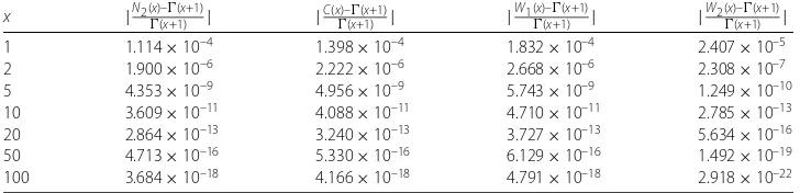
Table 1 Comparison amongN2(4.2),C(4.1),W1(1.3) andW2(1.6)

x _|N2(x)–(x+1)

(x+1) | |

C(x)–(x+1)

(x+1) | |

W₁₍x)–(x+1)

(x+1) | |

W₂₍x)–(x+1)

(x+1) |

1 1.114×10–4 1.398×10–4 1.832×10–4 2.407×10–5 2 1.900_×10–6 _2.222×10–6 _2.668×10–6 _2.308×10–7

5 4.353_×10–9 _4.956×10–9 _5.743×10–9 _1.249×10–10

10 3.609×10–11 _4.088×10–11 _4.710×10–11 _2.785×10–13

20 2.864×10–13 _3.240×10–13 _3.727×10–13 _5.634×10–16

50 4.713×10–16 _5.330×10–16 _6.129×10–16 _1.492×10–19

100 3.684×10–18 _4.166×10–18 _4.791×10–18 _2.918×10–22

and we have Windschitl one [13],

(x+ 1)∼√2πx

x e

x xsinh1

x+ 1 810x6

x/2

1 +O

1 x7

=W1(x).

For our new onesW2(x) given in (1.6) and its counterpartW2∗(x) given in (3.1), we easily

check that

lim

x→∞

ln(x+ 1) –lnW2(x)

x–9 =xlim→∞

ln(x+ 1) –lnW₂∗(x) x–9 =

869 2,976,750,

which show that the rates ofW2(x) andW2∗(x) converging to(x+ 1) are both asx–9.

From these, we see that our new Windschitl type approximation formulasW2(x) and

W₂∗(x) are best among those listed above, which can also be seen from Table 1.

Acknowledgements

The authors would like to express their sincere thanks to the editors and reviewers for their great efforts to improve this paper. This work was supported by the Fundamental Research Funds for the Central Universities (No. 2015ZD29) and the Higher School Science Research Funds of Hebei Province of China (No. Z2015137).

Competing interests

The authors declare that they have no competing interests.

Authors’ contributions

All authors contributed equally to the writing of this paper. All authors read and approved the final manuscript.

Author details

1_{College of Science and Technology, North China Electric Power University, Baoding, P.R. China.}2_{Department of Science}

and Technology, State Grid Zhejiang Electric Power Company Research Institute, Hangzhou, China.

Publisher’s Note

Springer Nature remains neutral with regard to jurisdictional claims in published maps and institutional affiliations.

Received: 12 December 2017 Accepted: 23 February 2018

References

1. Anderson, G.D., Vamanamurthy, M.K., Vuorinen, M.: Conformal Invariants, Inequalities, and Quasiconformal Maps. Wiley, New York (1997)

2. Anderson, G.D., Vamanamurthy, M.K., Vuorinen, M.: Topics in special functions II. Conform. Geom. Dyn.11, 250–270 (2007)

3. Wang, M.K., Chu, Y.M., Song, Y.Q.: Asymptotical formulas for Gaussian and generalized hypergeometric functions. Appl. Math. Comput.276, 44–60 (2016)

4. Wang, M.K., Li, Y.M., Chu, Y.M.: Inequalities and infinite product formula for Ramanujan generalized modular equation function. Ramanujan J. (2017). https://doi.org/10.1007/s11139-0176-9888-3

5. Wang, M.K., Chu, Y.M., Jiang, Y.P.: Ramanujan’s cubic transformation inequalities for zero-balanced hypergeometric functions. Rocky Mt. J. Math.46(2), 679–691 (2016)

6. Wang, M.K., Chu, Y.M.: Refinements of transformation inequalities for zero-balanced hypergeometric functions. Acta Math. Sci. Ser. B Engl. Ed.37(3), 607–622 (2017)

8. Gosper, R.W.: Decision procedure for indefinite hypergeometric summation. Proc. Natl. Acad. Sci. USA75, 40–42 (1978)

9. Batir, N.: Sharp inequalities for factorialn. Proyecciones27(1), 97–102 (2008)

10. Mortici, C.: On the generalized Stirling formula. Creative Math. Inform.19(1), 53–56 (2010) 11. Ramanujan, S.: The Lost Notebook and Other Unpublished Papers. Springer, Berlin (1988)

12. Smith, W.D.: The gamma function revisited (2006). http://schule.bayernport.com/gamma/gamma05.pdf 13. http://www.rskey.org/CMS/the-library/11

14. Mortici, C.: A new fast asymptotic series for the gamma function. Ramanujan J.38(3), 549–559 (2015) 15. Nemes, G.: New asymptotic expansion for the gamma function. Arch. Math. (Basel)95, 161–169 (2010) 16. Yang, Z.-H., Chu, Y.-M.: Asymptotic formulas for gamma function with applications. Appl. Math. Comput.270,

665–680 (2015)

17. Chen, C.-P.: A more accurate approximation for the gamma function. J. Number Theory164, 417–428 (2016) 18. Batir, N.: Inequalities for the gamma function. Arch. Math.91, 554–563 (2008)

19. Mortici, C.: An ultimate extremely accurate formula for approximation of the factorial function. Arch. Math.93(1), 37–45 (2009)

20. Mortici, C.: New sharp inequalities for approximating the factorial function and the digamma functions. Miskolc Math. Notes11(1), 79–86 (2010)

21. Mortici, C.: Improved asymptotic formulas for the gamma function. Comput. Math. Appl.61, 3364–3369 (2011) 22. Zhao, J.-L., Guo, B.-N., Qi, F.: A refinement of a double inequality for the gamma function. Publ. Math. (Debr.)80(3–4),

333–342 (2012)

23. Mortici, C.: Further improvements of some double inequalities for bounding the gamma function. Math. Comput. Model.57, 1360–1363 (2013)

24. Qi, F.: Integral representations and complete monotonicity related to the remainder of Burnside’s formula for the gamma function. J. Comput. Appl. Math.268, 155–167 (2014)

25. Lu, D.: A new sharp approximation for the gamma function related to Burnside’s formula. Ramanujan J.35(1), 121–129 (2014)

26. Lu, D., Song, L., Ma, C.: Some new asymptotic approximations of the gamma function based on Nemes’ formula, Ramanujan’s formula and Burnside’s formula. Appl. Math. Comput.253, 1–7 (2015)

27. Yang, Z.-H., Tian, J.F.: Monotonicity and inequalities for the gamma function. J. Inequal. Appl.2017, 317 (2017). https://doi.org/10.1186/s13660-017-1591-9

28. Alzer, H.: On some inequalities for the gamma and psi functions. Math. Comput.66(217), 373–389 (1997) 29. Yang, Z.-H.: Approximations for certain hyperbolic functions by partial sums of their Taylor series and completely

monotonic functions related to gamma function. J. Math. Anal. Appl.441, 549–564 (2016)

30. Alzer, H.: Sharp upper and lower bounds for the gamma function. Proc. R. Soc. Edinb.139A, 709–718 (2009) 31. Lu, D., Song, L., Ma, C.: A generated approximation of the gamma function related to Windschitl’s formula. J. Number

Theory140, 215–225 (2014)

32. Chen, C.-P.: Asymptotic expansions of the gamma function related to Windschitl’s formula. Appl. Math. Comput.245, 174–180 (2014)

33. Qi, F., Cerone, P., Dragomir, S.S., Srivastava, H.M.: Alternative proofs for monotonic and logarithmically convex properties of one-parameter mean values. Appl. Math. Comput.208(1), 129–133 (2009)

34. Tian, J.F., Ha, M.H.: Properties of generalized sharp Hölder’s inequalities. J. Math. Inequal.11(2), 511–525 (2017) 35. Tian, J.F., Ha, M.H.: Properties and refinements of Aczél-type inequalities. J. Math. Inequal.12(1), 175–189 (2018) 36. Abramowttz, M., Stegun, I.A.: Handbook of Mathematical Functions with Formulas, Graphs and Mathematical Tables.

Dover, New York (1972)

37. Yang, Z.-H., Chu, Y.-M., Tao, X.-J.: A double inequality for the trigamma function and its applications. Abstr. Appl. Anal. 2014, Article ID 702718 (2014)

38. Yang, Z.-H., Tian, J.: Monotonicity and sharp inequalities related to gamma function. J. Math. Inequal.12(1), 1–22 (2018)