© 2016, IRJET | Impact Factor value: 4.45 | ISO 9001:2008 Certified Journal
| Page 1966
A modified series solution method for fractional integro-differential
equations
Santanu Banerjee
1, Soumen Shaw
2, Basudeb Mukhopadhyay
3Department of Mathematics, Indian Institute of Engineering Science and Technology, Shibpur, India Email: 1[email protected]
2[email protected] 3[email protected]
---***---Abstract -
This paper is dealing with a modified series solution method for nonlinear fractional differential-integral equations. Based on the Caputo and Riemann-Liouville fractional derivatives some important theorems have been proved. Moreover, a one degree-of-freedom (dof) oscillator equation has been solved by using this new method. Finally, a comparison study is being made with the exact numerical solution.Key Words: Modified series solution method; fractional integro-differential equation; one degree-of-freedom oscillator equation; Caputo’s fractional derivative.
1.INTRODUCTION
In recent years fractional calculus draws considerably increasing attention due to its applicable uses in different fields of mathematics and science. Based on the past results of Nutting [1], Gemant [2] and Bosworth [3] were first proposed fractional derivative modeling for the constitutive behavior of viscoelastic media. Since then fractional calculus has been successfully applied in various fields of physics and engineering such as biophysics, bioengineering, quantum mechanics, finance, control theory, image and signal processing, viscoelasticity and material sciences. The use of these fractional derivatives and their application has in the last decade gained a noticeable improvement as shown by many peer-reviewed scientific papers, conferences and monograms.
The most important section of the fractional calculus in engineering and applied sciences is to find an analytic or approximate solution of fractional ordered initial or boundary value problems. Recently a great deal of interest has been focused on the solution of fractional differential equations (FDE) and fractional integral equations (FIE). FDE appears frequently in different research areas of applied science and engineering when we try to model a problem mathematically by considering derivatives of fractional order (see Ref. [4]). Apart from these fractional derivatives and integrals also appear in many physical problems such as frequency dependent damping behavior of materials, motion
of a large thin plate in a Newtonian fluid, creep and relaxation functions for viscoelastic materials, the PIλDμ
controller for the control of dynamical systems, etc(see Refs. [5-6]).
The solution FDE and FIE are complex since fractional derivatives and integrals of some common and frequently used functions are higher transcendental functions (see Ref. [7]). Most of the time it becomes difficult to get an exact solution of an FDE or FIE. Hence we tend to compensate an exact solution with an approximate series solution. For this we may sometimes get non-negligible numerical errors in solutions. So a reliable and efficient technique for the solution is very necessary.
It is almost true that most mathematical systems in real life problems are nonlinear in nature. In most of the times a common way of solving such nonlinear problems is to linearize the problem, where we replace the actual nonlinear system with a so called equivalent linear system and employ averaging which is in general not a good idea! Since linearization of a nonlinear problem may become grossly inadequate in some essentially real phenomenon. For example shock waves in gas dynamics can occur in nonlinear systems but cannot occur in linear systems. Thus a correct solution of a nonlinear system is very significant issue when we solve a nonlinear system rather than just linearizing the problem. If we want to know accurately how a physical system behaves in general then it is essential to retain the nonlinearity.
© 2016, IRJET | Impact Factor value: 4.45 | ISO 9001:2008 Certified Journal
| Page 1967
2. Mathematical Preliminaries
Fractional ordered derivatives have been encountered by several authors in different approaches (see Refs. [7,11]). In this paper we will focus on the Riemann-Liouville and the Caputo definitions since they are the most used once in applications.
The Riemann-Liouville approach is based on the Cauchy formula (2.1) for the nth integral which uses only a simple integration so it provides a good basis for generalization.
t
a
n t
a a a
n n
a
d
t
n
d
d
d
f
t
f
I
n
1
1 2 1
!
1
1
...
...
1 1
(2.1)
Now it is obvious how to get an integral of arbitrary order. We simply generalize the Cauchy formula (2.1)- the integer
n
is substituted by a positive real number
and the Gamma function is used instead of the factorial. Notice that the integrand is still integrable because
1
1
.
ta
a
f
t
t
d
I
1
1,
1
1
. (2.2) This formula represents the integral of arbitrary order0
, but does not permit order
0
which formally corresponds to the identity operator. This expectation is fulfilled under certain reasonable assumptions at least if we consider the limit
0
(for further details, see Ref. [5]). Hence, we extend above definition by setting
t
f
t
f
I
a
0
. (2.3)
The definition of fractional integrals is very straightforward and there are no complications. But for fractional derivative there is no such analogous to (2.1) so we have to generalize the derivatives through a fractional integral. First we perturb the integer order by a fractional integral according to (2.2) and then apply an appropriate number of classical derivatives. We can always choose the order of perturbation less than 1. The result of these ideas, the fractional derivative of a function f (t) of order α is defined as
ta n n
n n
a n n
a
t
d
dt
d
n
t
f
I
dt
d
t
f
D
t
f
D
1
1, where
n
1
. (2.4) The Caputo fractional derivative of a function f (x) of order α is defined as
x
f
dx
d
I
x
f
D
mm m
,
1
m
. (2.5) Here we shall always consider
0
and f (x) to bepiecewise continuous on
a
,
and integrable on any finite subinterval of
a
,
.The difference occurs for fractional derivative. A non-integer-order derivative is again defined by the help of the fractional integral, but now we first differentiate
f
x
in the common sense and then go back by fractional integrating up to desired order.It is essential to state that both the fractional integral and fractional derivative operators
D
andD
are linear in nature (see Ref. [3-4]), also for α,β>0,
D D
f x
D
f x
and
D D f x
D
f x
.
2.1 Generalized power series
In this paper we use the generalized power series
expansion
0
r
p r r
x
a
C
x
f
, wherep
is a fixed positive integer. The radius of convergence of this series isgiven by p
R
where1
lim
r r r
C
C
R
.3. Approaches from fractional derivative to
fractional ordered generalized power series
In this section we have proved some important theorems which will be essential to demonstrate the generalized power series.
Theorem: 1
© 2016, IRJET | Impact Factor value: 4.45 | ISO 9001:2008 Certified Journal
| Page 1968
1
1
1
m n
n m
r n
n m r m
x a r n
D
D f x
D
f x
D
f x
x a
r
n
Proof: We know,
x a x a x a m mdx
x
f
x
f
D
....
Therefore,
x a x a x a m n m ndx
x
f
D
x
f
D
....
1 1 2 2 1...
1
2
mn m n
m n
n m n m
x
a
D
f x
D
f a
m
x
a
D
f a
m
x
a
D
f a
D
f a
11
m r mn m n r
r
x
a
D
f x
D
f a
m
r
(3.1)By changing the range of summation from r = 1(1)m to r = n(1)n+m-1 in the term on the right hand side of equation (3.1), we get,
m n
D D f x
1
1
r m n m r n n m r nD
f a
D
f x
x
a
r
n
(3.2)In Particular: When m = n, equation (3.2) reduces to,
1
0
1
r n r n n rD f a
D D f x
f x
x
a
r
(3.3) Lemma: 1The Riemann-Liouville fractional integral of the generalized power series is given by,
0 01
1
r p r r r p rr
x
a
p
r
p
r
c
a
x
c
I
,
where
r
p
0
.Proof: Considering the linear nature of the fractional integral operator and by going on the definition of the Riemann-Liouville fractional integral we get,
0 r p r rx
a
c
I
10 0
1
(
)
(
)
( )
r x p r rx
t
c t
a
dt
(3.4)Then by making the substitution
t
a
x a
in the right side of equation (3.4) and using the integral definition of beta function we obtain,
0 r p r rx
a
c
I
0
(
)
,
1
,
1
0
( )
r p r
r
c
r
r
x
a
B
where
p
p
01
,
0
1
r p r rr
p
c
x
a
where r
p
r
p
(3.5) Lemma: 2The fractional order derivative of the generalized power series is given by,
0 01
(
)
1
r r p p r r r rr
p
D
c x
a
c
x
a
r
p
,where
r
p
0
(3.6)Proof: By merely applying the definition and linear property of the Riemann-Liouville fractional integral and fractional derivative we get,
0
(
)
r p r rD
c x
a
(1 ) 0(
)
r p r rDD
c x
a
© 2016, IRJET | Impact Factor value: 4.45 | ISO 9001:2008 Certified Journal
| Page 1969
10
1
2
r p r rr
p
D
c
x
a
r
p
01
1
r p r rr
p
c
x
a
r
p
, wherer
p
0
.(3.7)
Theorem: 2
The Riemann-Liouville fractional integral and fractional derivative of the generalized power series are mutually commutative in nature i.e.,
0 0
(
)
(
)
r r p p r r r rD D
c x
a
D D
c x
a
,where
r
p
0
.Proof: Applying fractional ordered integral and differential
operators taken upon the series 0
(
)
r p r rc x
a
and Using the Lemma-1 and Lemma-2 we get,0
(
)
r p r rD D
c x
a
01
1
r p r rr
p
D
c
x
a
r
p
01
1
r p r rr
p
c
D
x
a
r
p
01
1
r p r rr
p
c
x
a
r
p
. Similarly, 0(
)
r p r rD D
c x
a
01
1
r p r rr
p
D
c
x
a
r
p
01
1
r p r rr
p
c
x
a
r
p
Thus, 0(
)
r p r rD D
c x
a
= 0(
)
r p r
r
D D
c x
a
(3.7)Hence the result follows.
It will be important for the following sections to note that in the above result (3.7) apart from being pure fractions, both α and β can be integers also. Also it will be important to note that all the above results depicted are still true if we consider the definition of fractional derivative given by Caputo because the basic difference between the definitions of Riemann-Liouville and Caputo is that in the former integration is followed by differentiation whereas in the later differentiation is followed by integration.
4. Main results
Let us consider a general version of a nonlinear fractional integro-differential equation of the form:
x
f
Ny
y
D
y
D
Ry
y
D
n
,
nn
a
a
y
D
a
a
Dy
a
a
y
1,
2,
....
(4.1)where ,Dn
1 2 1
1 2 1
,
..
..
..
n n
x x x x
n
n
n n
a a a a
d
D
dt dx dx dx
dx
© 2016, IRJET | Impact Factor value: 4.45 | ISO 9001:2008 Certified Journal
| Page 1970
D
fractional differential operator,
D
fractional integral operator,
N
nonlinear operator.By applying D-non both sides in equation(4.1) we get,
y=
( )0
( )
1
r n
r r
x
a
y
a
r
+D-nf-D-nRy-D-nDαy-D-nD βy-D-nNNow we consider,
0
r p r
r
y
c x
a
,
0
r p r
r
f
f
x
a
and
0
( )
r p r
r
N y
B x
a
where p can be any positive integer according to the requirement of the problem (The selection of p will entirely depend upon the function f), so that we get
0
0 0
0 0
0 0
1
r p r
r
r
n r
n p
r r
r r
r r
n n
p p
r r
r r
r r
n p n p
r r
r r
c
x a
x a
a
D
f
x a
r
D
R
c
x a
D
D
c
x a
D
D
c
x a
D
B x a
(4.2) By applying the Lemma-1, Lemma-2 and Theorem-1, Theorem-2in the above equation (4.2) and by also considering the linear property of the differential and integral operators we obtain,
1 0
0
1
1
1
r
np r
p p
r r
r r np n
r r
r
r r np r np r np
p r np r np r np
c x
c x a
a
x a
r
r
n
f
Rc
D c
p
x a
r
D c
B
p
(4.3)
Equating the coefficients from both sides of equation (4.3) we calculate the values of
c
rusing the recurrence relations obtained and hence find the solution
0
r p r
r
y
c x
a
.5. Applications:
Power series solutions of linear homogeneous differential equation in one-point boundary value problems yield simple recurrence relations for the coefficient, but in most of the cases they are generally seen not to be adequate for nonlinear equations. A reliable modification in the terms of the series solution can yield good results for nonlinear non homogeneous differential equations. In fact we can use this modification on the series solution to get good results for nonlinear non-homogeneous fractional differential equations also.
To clarify this let us consider the following motion equation of a one-degree-of-freedom oscillator
mD2y + c
1 2
D
y + ky2 = f(x) ,y(0)=0 , Dy(0)=0 ,(5.1)
where,
7 5 3
2 2 2 2
2 2
3
8
3
8
2
4
4
10
10
10
10
8
128
88
16
2
35
25
25
10
3
8
10
10
f x
x
x
x x
x x
x
x
x
x
x
x
x
Here we consider p=2 , so that
2 0
r r r
y
c x
, 20
r r r
f
f x
, and,2 0
( )
r r r
N y
B x
Thus from equation (5.1) we get,
1
2 2 2 2 2
1
(0)
(0)
c
k
y
y
xy
D
f
D D y
D y
m
m
m
or,
2
2 2
0 0
1
2 2 2 2 2
0 0
1
r r
r r
r r
r r
r r
r r
c x
D
f x
m
c
k
D
D
c x
D
B x
m
m
© 2016, IRJET | Impact Factor value: 4.45 | ISO 9001:2008 Certified Journal
| Page 1971
or,2
1 2
2 2
0 0
1
1
2
2
2
r r
r r r r
r r
c
k
x
c x
f
c D
B
r
r
m
m
m
Therefore,
1 3
2 2 2
0 1 2 3
4
r r r
c
c x
c x
c x
c x
1
2 2
4 4 4
4
4
1
2
r
r r r
r
c
k
f
c
D
B
x
r r
m
m
m
(5.2)Comparing both sides of equation (5.2) we get,
0 1 2 3
0
c
c
c
c
1 2
4 4 4
4
1
,
4
2
r r r r
c
k
c
f
c
D
B
r
r r
m
m
m
(5.3)
Now,
2 0
r r r
f x
f x
gives,1 3
2
2 2
0 1 2 3 4
5 7 9
3 4
2 2 2
5 6 7 8 9
7 5 3
2 2 2 2
2 2
...
3
8
3
8
2
4
4
10
10
10
10
8
128
88
16
2
35
25
25
10
3
8
10
10
f
f x
f x
f x
f x
f x
f x
f x
f x
f x
x
x
x x
x x
x
x
x
x
x
x
x
Comparing, we get,
0 1 2 3 4
5 6 7 8
12
33
64
,
0,
,
,
12,
25
5
125
352
512
4
,
0,
,
625
125
175
f
f
f
f
f
f
f
f
f
Using equations (5.3) we obtain
0
0
c
1 2
1
0
c x
2
0
c x
3 2
3
0
c x
1
2 2 2 2
4 0 0 0
4
1
6
4 4 2
25
c
k
c x
f
c D
B
x
x
m
m
m
m
5 1 5
2 2 2
5 1 1 1
4
1
0
5 5 2
c
k
c x
f
c D
B x
m
m
m
1
3 2 3 3
6 2 2 2
4
1
11
6 6 2
10
c
k
c x
f
c D
B
x
x
m
m
m
m
7 1 7
2 2 2
7 3 3 3
7 2
4
1
7 7 2
256
4375
c
k
c x
f
c D
B
x
m
m
m
x
m
1
4 2 4
8 4 4 4
7
4 2
2
4
1
8 8 2
1
64
875
c
k
c x
f
c D
B
x
m
m
m
c
x
x
m
m
...
Thus the solution is given by
1 3 5
2 3
2 2 2
0 1 2 3 4 5 6
7 4 2
7 8
...
y
c
c x
c x c x
c x
c x
c x
c x
c x
7
2 3 2
2 4
6
11
256
64
25
10
4375
875
1
...
c
x
x
x
m
m
m
m
x
m
By considering the first nine terms only we get,
2 3 722 4
6
11
256
64
25
10
4375
875
1
c
y x
x
x
x
m
m
m
m
x
m
© 2016, IRJET | Impact Factor value: 4.45 | ISO 9001:2008 Certified Journal
| Page 1972
6. Numerical results and discussion:
In the following numerical computation we have assumed m=1, c=0.8, and k=1.According to [12] considering m=1, c=0.8, and k=1 the exact solution is,
23
8
10
10
y x
x
x
x
(6.1)An approximate solution of equation 5.1) was also obtained by Sutradhar et. al. [10] using a modified decomposition method and then compared with the exact solution as given by Wang Ji-Zeng et al. [12]. The approximate solution of equation (5.1) as obtained by Sutradhar et. al. [10] is,
11 9 7
10 9 8 7 6 3 2 2 2 2
4
1 11 169 11 6 11 6 1 2048 1408 256 ( )
90 360 5600 875 3125 10 25 17325 7875 4375
x x x x x x x x x x
y x x
m
7
2 2
2
5
32 6 2 11 8 8 6 14 11 16 169 6 11 2
1
25 3 10 11 13 3125 17 875 19 5600 7 360 207
105
7 256 3 1408 1024
128 4375 4 7875 11025
c x x x x x x x x
m
x x x
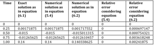
(6.2) Under the assumptions m=1, c=0.8, and k=1 in equation (5.1), the following table shows the comparison of the approximate numerical solutions given in equations (5.4) and (6.2)with the exact solution given in the equation (6.1). It is interesting to note that the numerical solution obtained in our case coincides with the exact numerical solution.
Table 1. : Considering the solution given in the equation (5.4) and in the equation (6.2)(Taking m=1, c=0.8 and k=1)
Time Exact solution as in equation (6.1)
Numerical solution as in equation (5.4)
Numerical solution as in equation (6.2)
Relative error considering equation (5.4)
Relative error considering equation (6.2)
0 0 0 0 0 0
0.25 0.00171875 0.00171875 0.001717552 0 0.000697147 0.50 -0.015 -0.015 -0.015011315 0 0.000754321 0.75 -0.01265625 -0.01265625 -0.012610457 0 0.003618248 1.00 0.14 0.14 0.140338625 0 0.00241875
From the above two tables we observe that our approximate solution considering 9-terms is in a far better agreement with the exact solution than the solution in equation (6.1) which considers far many terms compared to ours.
7. Conclusion:
Nonlinear problems play a crucial role in applied mathematics and physics. In maximum of the cases these nonlinear problems are tackled by the methods which propose to linearize the given nonlinear problem. Such approach not only hampers the solution process partially but also sometimes misinterprets the actual nature of the problem. There are a very few proposed methods which solve nonlinear equations without linearizing the problem. In this paper we illustrated a generalized power series method for solving a nonlinear problem very easily and elegantly and that too without linearizing the problem.
We proposed and illustrated an efficient modification of the power series for getting an approximate series solution of a nonlinear fractional integro-differential equation. The motive of using a fractional power in the power series can be raised. It is due to the fact that we always proceed by equating like terms in such methods, and if the function f (x) in say equation (5.1) contains fractional powers of x then our consideration of the generalized power series can yield better results. The present analysis also shows that the computational procedure in our method is simple and is based on recursion. The obtained results show that although other methods are available, the present method produces very promising solutions without availing any difficulty. Here we also compared our result with the exact solution as obtained in [12] and an approximate solution as obtained in [10]. We observed that our numerical solution almost identical with the exact solution whereas the solution given by Sutradhar et al [10] had relative errors when compared with the exact solution. Thus, to solve the similar types physical problems which has been considered in the present analysis, this method is more appropriate than other generalized series solution approaches.
References:
[1] P.G. Nutting, A new general law deformation, J. Franklin I. 191 (1921) 678-685.
[2] A. Gemant, On fractional differentials, Philos. Mag. Ser. 25 (1938) 540-549.
[3] R.C.L. Bosworth, A definition of plasticity, Nature. 157 (1946) 447.
[4] S.P.Näsholm, S.Holm (2011). Linking multiple relaxation, power-law attenuation, and fractional wave equations. Journal of the Acoustical Society of America 130(5), pp. 3038-3045.
[5] L.E.Suarez, A.Shokooh (1997). An eigen vector expansion method for the solution of motion containing fractional derivatives. Transaction ASME Journal of Applied Mechanics 64(3), pp.629-635.
[6] W.G.Glockle, T.F.Nonnenmacher (1991). Fractional integral operators and fox functions in the theory of viscoelasticity. Macromolecules 24, pp.6426-6434.
[image:7.595.34.291.465.541.2]© 2016, IRJET | Impact Factor value: 4.45 | ISO 9001:2008 Certified Journal
| Page 1973
[8] S.SahaRay, R.K.Bera (2006).Analytical solution of afractional diffusion equation by Adomain decomposition method. Appl. Math. Comput174, pp.329-336.
[9] M.S.Mohamed (2014). Optimal homotopy analysis method for solving time space nonlinear partial fractional differential equations. IJAMM 10(12), pp.1-9.
[10] T.Sutradhar, B.K.Datta, R.K.Bera (2012).Analytic solution of time fractional nonlinear dynamic system by modified decomposition method.International Journal of Applied Mechanics and Engineering 17(4), pp.1327-1337.
[11] I.Podlubny (1999). Fractional differential equations.Academic Press.