High fidelity imaging and high performance computing in
nonlinear EIT
B H Blott†, S J Cox‡, G J Daniell†, M J Caton‡ and D A Nicole‡
† Department of Physics and Astronomy, University of Southampton, Southampton SO17 1BJ, UK
‡ Department of Electronics and Computer Science, University of Southampton, Southampton SO17 1BJ, UK
Received 16 July 1999
Abstract. We show that nonlinear EIT provides images with well defined characteristics when smoothness of the image is used as a constraint in the reconstruction process. We use the gradient of the logarithm of resistivity as an effective measure of image smoothness, which has the advantage that resistivity and conductivity are treated with equal weight. We suggest that a measure of the fidelity of the image to the object requires the explicit definition and application of such a constraint. The algorithm is applied to the simulation of intra-ventricular haemorrhaging (IVH) in a simple head model. The results indicate that a 5% increase in the blood content of the ventricles would be easily detectable with the noise performance of contemporary instrumentation. The possible implementation of the algorithm in real time via high performance computing is discussed. Keywords: nonlinear electrical impedance tomography, intraventricular haemorrhaging, parallel computing, inverse problem constraints
(Some figures in this article appear in black and white in the printed version.)
1. Introduction
Linear image reconstruction in EIT has been widely used in medical and process applications, and nearly all of these have been based on approximately uniform distributions of the electrical conductivity in the object under study. Successful applications in medicine have been reported (Holder 1993) although the markedly non-uniform conductivity distribution in the human body, which is not known a priori, means that artefacts produced by the linear imaging approximation are difficult to exclude. It is important therefore to pursue the full nonlinear problem in order to provide robust imaging as well as provide a firm basis for subsequent linear treatments. We have already shown (Blott et al 1998) that effective nonlinear EIT can be achieved when appropriate choices are made to constrain the form of the images sought and have applied the method to real experimental data. In this paper we further demonstrate the properties of our algorithm and apply it to a simple model of intra-ventricular haemorrhaging in the neo-natal head (Zadehkoochak et al 1991). We conclude with an outline of the potential application of parallel computing in EIT to allow nonlinear reconstruction in practicable time scales.
2. Essential properties of EIT reconstruction
In recent years considerable effort has been devoted to devising reconstruction algorithms for electrical impedance tomography that are fast (see for example Pinheiro and Dickin 1997) in order to produce images in real time. In contrast, in this paper we focus attention on the nature of the images produced whilst still demanding that those images can be produced in acceptable time scales. It is crucial to recognize that we are dealing with an inverse problem, that is, constructing a continuous resistivity distribution, with an infinite number of variables, from a finite dataset. Unlike other imaging methods, even large changes in conductivity restricted to a small region in the interior of the body produce only small changes in the measured data. Since the data inevitably contain noise these large but very localized changes in conductivity are undetectable. Another way of putting this is that many images are consistent with a given data set and these differ fairly grossly in the fine details. The image reconstruction method used has to recognize this fact.
A nonlinear reconstruction algorithm aims to construct a resistivity distribution that would lead to the potential differences that are actually observed. The agreement is usually expressed by a particular value of theχ2statistic defined by
χ2=X i
(Vi(predicted)−Vi(observed))2 σ2
i
. (1)
Hereσi is the error in measurementVi. The agreement between theory and experiment is usually regarded as satisfactory ifχ2is approximately equal to the number of observations: that is the observations are expected to be not more than one standard deviation in error on average. Some strong prior evidence would be required to accept a prediction that led to a value ofχ2either much less or much greater than the number of values in the data.
We take the measure of random noiseσias the unavoidable instrumentation noise in making the measurement of the transimpedance, added to which there may be unwanted signals picked up from the environment. In the resulting image there will of course be random and systematic uncertainties arising from the physiology under study (Meeson et al 1996). It is preferable to deal with this explicitly during subsequent image analysis.
We now need a criterion to select one of the many images that fit the data within the agreed tolerance. An important point is that the decision should be based on some property of the image so that explicit image characteristics are the focus of the reconstruction process. The obvious criterion is to select the image that minimizes or maximizes some property of the resistivity or conductivity distribution. Our rule for defining the EIT image is to minimize
Z
image
"
∂logρ ∂x
2 +
∂logρ ∂y
2#
dxdy+λχ2. (2)
This gives the image with the least mean square gradient of logρ, while the Lagrange multiplier
λenables us to constrainχ2to equal the number of values in the data. There is no fundamental reason to make a distinction between resistivity and conductivity in the reconstruction. Our use of the logarithm of the resistivity achieves this desirable property, since logσ = −logρ. This constraint has been used successfully by others including Barber et al (1984) and Adler
et al (1996).
3. Numerical method
the solution should not depend on the numerical algorithm. For any realistic signal-to noise ratio the resistivity distributionρ(x, y), defined by minimizing (2), is a fairly smooth function whose spatial scale is fixed by the patterns of current flow which are intrinsic to the measuring apparatus and the object under study. For computational purposes it is important that the image pixels are small enough so that this intrinsic resolution is achieved and no systematic errors introduced.
Our numerical work has used a standard 2D finite element model (FEM) to solve the generalized Laplace equation (Silvester and Ferrari 1983). Following other workers we ignore the derivative of the Jacobian which is computationally expensive to calculate. Although the first term in (2) means that the problem is less ill conditioned it is still necessary to add a constant to the diagonal of the matrix of second derivatives to make the iteration stable when
λis large (see Vad´asz and Sebesty´en 1996). The constantλis adjusted by trial and error to produce solutions with particular values ofχ2.
The full nonlinear solution relies on calculation of the sensitivity Jacobian, which determines the effects of local changes in the conductivity on the observed measurements. This matrix can therefore be used to determine the local maximum resolution which can be produced by the instrumentation in a specific application. In particular it is possible to exploit self-adapting finite element techniques to ensure that the mesh used for the computation does not itself affect the quality of the image produced: only the quality of the data and the constraints applied determine the resulting image. This constrasts with the approach employed by Cheney
et al (1990). It is imperative that the adaption of the mesh should be performed as the nonlinear
solution progresses, not at the outset of the calculation. This dynamic refinement allows the quality of the mesh to be determined by, for example, the local gradient of the conductivity, ensuring that the mesh is tuned to the image which is being reconstructed.
0 5
10 15
0 5 10 15 0 1 2 3
0 1 2 3
0 4
8 12
16
0 4 8 12 16
0 1 2 3
[image:3.595.104.456.406.656.2]0 1 2 3
5 10 15 2
4
6
8
10
12
14
16
−6 −4 −2 0
0 4
8 12
16
0 4 8 12 16 −5 −4 −3 −2 −1 0
−6 −4 −2 0
Figure 2. A simplified head section showing conductivity of scalp, skull, white matter and ventricles
on a log scale.
A frequent objection to the Newton–Raphson algorithm in its simplest form is that it involves the inversion of a matrix whose size is the large number of image pixels. However, by using the Woodbury formula (Press et al 1992), it is only necessary to invert a matrix whose size is determined by the number of data values. It is also possible to employ Arridge’s adjoint source method (1999) or to use an iterative inversion method. Therefore the use of a locally fine mesh to ensure a high fidelity image is not an impediment to a fast reconstruction.
4. Results from a test object
Figure 1 shows the statistically optimal images produced by data from a square pillar test object on a relatively coarse grid. Although the images are true to the data they do not show high fidelity to the generating object, since the gradient constraint smoothes out discontinuities in the object. This is a direct and explicit result of the chosen constraint: other choices will result in different images. The choice of constraint needs to be informed by the kind of image which clinicians find diagnostically useful.
5. Intra-ventricular haemorrhaging (IVH) in a simple head model
0
4
8
12
16
0
4
8
12
16
0
0.5
1
100% CSF
0 0.2 0.4 0.6 0.8 1
0
4
8
12
16
0
4
8
12
16
0
0.5
1
100% Blood
[image:5.595.102.465.80.370.2]0 0.2 0.4 0.6 0.8 1
Figure 3. Image of ventricular region of interest (ROI) showing ventricles full of cerebro-spinal
fluid (left) or blood (right).
0 20 40 60 80 100
25 30 35 40 45 50
% Blood in Ventricles
Total Resistivity over ROI
Figure 4. Total resisitivity summed over the 20 pixel region of interest as a function of the volume
fraction of blood in the ventricles. We have assumed a noise to signal ratio of 10−3.
[image:5.595.156.392.417.606.2]0 100 200 300 400 500 600 700 800
1 2 3 4 1 2 3 4
No processors
T
ime (sec
s)
Stage 4
Stage 3 (parallel section) Stage 2
Stage 1
PII 266MHz (10MBit ethernet)
DEC Alpha 500MHz (100 MBit ethernet)
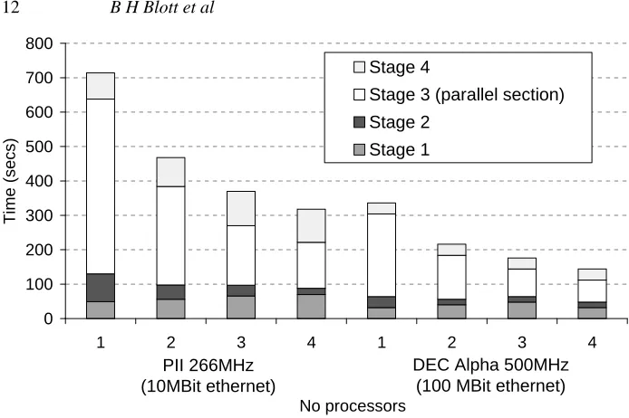
Figure 5. Parallel performance of a commercial finite element code running on commodity
processors showing increased speed as more processors are used in the calculation. (Left) Pentium nodes. (Right) DEC Alpha nodes.
data contained a random noise component of 0.1% of the maximum signal, which is achievable with available measurement systems. From the results a blood volume fraction change of 5% is easily detectable. In this application it is an increase in blood which must be detected, so any constant systematic errors in the nonlinear image would be eliminated. Furthermore it is likely that a fast linearized method would be satisfactory for small deviations from the full nonlinear reconstruction.
6. High performance computing
For the study of IVH, each 20% increment in the resistivity of the ventricular region of interest required three steps of the Newton–Raphson imaging procedure to refit the data. It is possible to improve the performance of the full nonlinear reconstruction using parallel computing. In figure 5 we show some typical results of the speedup of a finite element code (actually used for loudspeaker design!) on cheap commodity processors running Windows NT. Only the most expensive part of the computation is parallelized, and the time taken to execute this part decreases as more processors are added. However an inherently sequential part of the code remains which limits the efficient scalability of the code to between four and eight processors. In the figure we see that good speedup can be obtained using four Intel-based nodes. A total speed up of a factor of 10–20 over the performance of a desktop Intel machine can be obtained by using a small number of fast Alpha-based processors, which benefit from enhanced clock speed and superior floating point performance.
7. Conclusions
[image:6.595.95.442.76.307.2]to be used. With the choice of a logarithmic function the resulting images are invariant to the scale of the resistivities and to the interchange of resistivity and conductivity. A standard finite element approach coupled with a Newton–Raphson solver provides an effective numerical algorithm to solve the full nonlinear reconstruction problem. The simulation of intra-ventricular haemorrhaging in a simple head model indicates that a 5% increase in the blood content of the ventricles would be easily detectable with the noise performance of currently available instrumentation. We plan in future work to use parallel computing and self-adapting meshes in our finite element code to improve the speed of the nonlinear reconstruction and to obtain optimal resolution for a given signal-to-noise performance. We will apply this improved algorithm to real experimental data. Our constrained nonlinear reconstruction extends naturally to three dimensions.
References
Adler A and Guardo R 1996 Electrical impedance tomography: regularized imaging and contrast detection IEEE
Trans Med. Imaging 15 170–9
Arridge S R 1999 Optical tomography in medical imaging Inverse Problems 15 41–93
Barber D C, Brown B H and Freeston I L 1984 Information Processing in Medical Imaging ed F Deconinck and M Nijhoff (Dordrecht: Kluwer) pp 446–62
Blott B H, Daniell G J and Meeson S 1998 Nonlinear reconstruction constrained by image properties in EIT Phys.
Med. Biol. 43 1215–24
Cheney M, Isaacson D, Newell J C, Simske S and Goble J 1990 NOSER: an algorithm for solving the inverse conductivity problem Int. J. Imaging Syst. Technol. 2 66–75
Holder D (ed) 1993 Clinical and Physiological Applications of Electrical Impedance Tomography (London: UCL Press)
Meeson S, Blott B H and Killingback A L T 1996 EIT data noise evaluation in the clinical environment Physiol. Meas.
17 (suppl) A33–A38
Pinheiro P A T and Dickin F J 1997 Sparse matrix methods for use in electrical impedance tomography Int. J. Numer.
Methods Eng. 40 439–51
Press W H, Flannery B P, Teukolsky S A and Vetterling W T 1992 Numerical Recipes in C 2nd edn (Cambridge: Cambridge University Press) pp 74–7
Silvester P P and Ferrari R L 1983 Finite Elements for Electrical Engineers (Cmbridge: Cambridge University Press) Vad´asz D and Sebesty´en I 1996 Comparison of the Newton–Raphson and the spectral expansion impedance
tomography reconstruction algorithms IEEE Trans. Magn. 32 1286–9
Zadehkoochak M, Blott B H, Hames T K and George R F 1991 The spectral expansion of a head model for EIT Clin.