Online Full Text



Abstract—The use of computational fluid dynamics (CFD) to

solve the Reynolds-Averaged Navier-Stokes (RANS) equations in vertical axis wind turbine (VAWT) systems has been remarkably helpful in the performance improvement of VAWTs. In this study, the k-ω SST turbulence model was used to predict the steady wind flow performance of a 5kW three-bladed H-rotor Darrieus VAWT with cambering and tubercle leading edge (TLE) incorporated in the blades. TLE modification on a cambered airfoil VAWT was shown to be detrimental to flow and performance using torque, lift and drag data. These were further verified using the vorticity profiles showing the z-vorticity and Q-criterion where the baseline cambered VAWT was shown to have streamlined flow generally throughout one full VAWT rotation while the TLE VAWT generated explicitly massive vortices the size of the blade chord at blade wakes between azimuthal positions of 106° and 180° that induced drag increase and torque reduction. Between θ = 55° to 186°, negative torque values up to -3.59Nm were monitored. These negative torques coupled with the reduced lift sufficiently caused the overall performance degradation. The TLE blade in the VAWT generated turbulence instead of containing or decreasing it. Unlike the cambered VAWT that harnessed 41.6W of the 137.8W available wind power, the TLE VAWT generated only 9.28W of power.

Index Terms— TLE, Camber, VAWT, CFD

I. INTRODUCTION

NTEREST on vertical axis wind turbines (VAWTs), which has research initiatives stalled in the 1990s is currently re-emerging, with the United States focusing on large-scale offshore installations and researchers eyeing the inherent advantages of VAWTs, namely, accepting wind from any direction, fitting near ground installation, and thus having simpler design, construction and operation [1],[2]. With research and development on VAWTs gaining momentum, much focus has been on its performance improvement, in which this study is also anchored on.

Generally, experimental modeling and/or computational methods are used to study VAWT performance. Computational methods are either with panel codes or

This work was supported in part by the Department of Science and Technology (DOST) of the Republic of the Philippines under the Engineering Research and Development for Technology (ERDT) Program.

I. C. M. Lositaño, B.Sc. is a M.Sc. student of the Energy Engineering Program, University of the Philippines Diliman.

L. A. M. Danao, Ph.D. is an Associate Professor of the Department of Mechanical Engineering, University of the Philippines Diliman (corresponding author, e-mail: [email protected]).

Navier-Stokes (N-S) codes. The latter computational method also known as computational fluid dynamics (CFD) numerically solves the mass conservation and momentum equations in three dimensions – the N-S equations – as a function or not of time [3]. While an exact solution to the N-S equations does not exist, the CFD solution is time- or Reynolds-averaging, which CFD solvers accomplish using models like the two-equation eddy-viscosity k-ω shear stress transport (SST) turbulence model, an apt choice of CFD turbulence model for VAWTs because it provides detailed and accurate information in near-wall regions while allowing freestream independence in the farfield by combining the k-ω turbulence model best for wall-bound flows and the k-ɛ turbulence model featuring freestream turbulence [4].

Using pitching airfoil study, Edwards et al [5] have shown the k-ω SST turbulence model to ably predict airfoil experimental behavior. In VAWT performance studies, 2D CFD models have been generally found to correctly duplicate experimental results although significantly outperforming it and 3D counterparts [1],[6]. The study of Howell et al [1] even predicted the 3D CFD performance coefficient to be lower than the experimental due to the over tip vortices observed in the 3D simulation. For the same reason, the 2D CFD results of Castelli et al [6] are proportionately better than the wind tunnel test. Over tip vortices were disregarded in the 2D simulation.

The VAWT mesh and geometry are concerns in effecting simulation results. With their mesh convergence study, Zadeh et al [7] showed the mesh quality correlating with convergence: the finer the mesh, the more accurate the solutions and refined the flow visualizations were. Meanwhile, Castelli et al [6] proved the y+ _{as blade}

near-mesh quality indicator for VAWTs to configure the appropriate 2D and 3D meshes and corresponding turbulence model: y+ _{= 30 for k-ω SST turbulence model}

and y+ _{= 1 for Enhanced Wall Treatment k-ɛ Realizable.}

Bourguet et al [8] performed multi-criteria optimization to obtain the shape design of a VAWT airfoil using Design of Experiment/Response Surface Methodology (DOE/RSM) where a profile yielded was close to the National Advisory Committee for Aeronautics (NACA) 0025 airfoil profile. Howell et al [1] found that higher solidity VAWTs performed better over most of the operating range and that blade pitch angle changes, however small, deteriorated turbine performance because of dynamic stalling, which causes rapid and large fluctuations in rotor forces and torques.

The Performance of a Vertical Axis Wind

Turbine with Camber and Tubercle Leading

Edge as Blade Passive Motion Controls

Ian Carlo M. Lositaño, and Louis Angelo M. Danao,

Member, IAENG

NACA 1425 three-bladed H-rotor Darrieus VAWT in unsteady wind. Rolin and Porté-Agel [10] reported a VAWT with blade profiles having 5% circular arc camber having better lift-to-drag ratios and delayed stall at low Reynolds numbers. Using Blade Element Momentum (BEM) Model, Battisti et al [11] studied different small VAWT architectures in terms of performance and loads where one conclusion was that the cambered airfoil DU 06-W-200 showed increased rotor performance at starting TSRs, and increased torque and thrust values. Using k-ɛ RNG turbulence model in CFD, Loya et al [12] showed cambering up to 3% to increase VAWT blade torques due to changing pressure differential around the airfoil but decrease it beyond 3% due to increased turbulence and flow separation.

Tubercles as shown in Fig. 1 are naturally occurring bumps in humpback whale flippers acting as vortex generators that aid in the motion of these mammals in water by lift-induced drag [13]. There are other theories as to how tubercles operate in whale flippers although this is the most accepted. (Show flipper physiology). Two decades ago, Fish adopted the tubercles into airfoils with the tubercle leading edge (TLE), which led to comprehensive studies in tidal applications and HAWTs [14],[15]. WhalePower Corporation reported 25% improvement in airflow and 20% in power production of its TLE-modified HAWTs [13]. In another study, a NACA 63-021 airfoil with TLE was shown to increase the maximum lift by 4.8%, lift-to-drag ratio by 17.6%, decrease induced drag by 10.9% at an AOA of α = 10˚ [16]. TLE has been observed to influence laminar separation or bubble formation near the leading edge, dynamic stall and tonal noise in airfoils [17],[18]. Hansen [17] furthered that TLE in airfoils increased the lift in post-stall flow regime but sometimes at the expense of lift in pre-stall, but that this can still be refuted by keeping the amplitude-to-wavelength ratio, A/W, low. Wang and Zhuang [19] and Bai et al [20] seconded this conclusion with CFD results.

In standalone airfoils, TLE increases lift and stall angle, reduces drag to delay separation, and minimizes tip stall to restrict spanwise flow. Corsini et al [21] showed TLE in cambered airfoils to cause earlier post-stall recovery and lift gain. Pressure isolines were shown to have no separation in the spanwise direction for cambered profiles.

In VAWTs, results are conflicting. At low Reynolds number and low TSR range, a two-bladed NACA 0018

H-differences, both studies had different discretized 3D domains. Wang and Zhuang [19] modeled the blade tips of the VAWT geometry while Bai et al [20] limited the portion of the geometry and mesh under study to one full wavelength or one crest and trough combination in all three blades taking each blade as a unit component or infinitesimal part of a continuously long blade, thus ignoring tip vortices generated at the blade ends.

TLE effects on VAWT performance still needs further research. In this study, the performance effects of TLE on a three-bladed NACA 1425 H-rotor Darrieus VAWT in steady wind are carefully elaborated on.

II. METHODS

Computer-aided design (CAD) and computer-aided engineering (CAE) software were used to model the VAWT, run pressure-based transient numerical simulations on the model to quantify wind flow parameters needed to compute CP values and other derived quantities, and conduct post

processing for the comparative performance analyses between the baseline VAWT with cambered airfoils (cambered) and VAWT with cambered and TLE airfoils (TLE).

CAD was used to construct the geometry models from which the fluid environment was meshed. Model scale is 1:1. The model was validated in terms of performance against experimental and CFD data of similar 5 kW capacity three-bladed NACA XX25 H-rotor Darrieus VAWTs.

To optimize the CFD model, parametric studies on the y+_,

blade node density and time step were performed on the 2D model. The y+ _{study resolved the boundary layer}

requirements of near-wall cells, particularly the cell meshes surrounding and nearby blade surfaces. The node density study determined a suitable if not optimal cell size distribution near the critical areas of flow, which are the cells near and adjacent to the leading and trailing edges of the blades. The time step study, furthermore, optimized the temporal distribution of the wind flow across the VAWT. The resulting spatial and temporal discretization from the parametric studies were then factored into the 3D model.

Solver ANSYS® _Fluent® _{was used for the CFD}

simulations in a 64-bit desktop computer with four physical cores and eight threads operating up to 3.4 GHz frequency, and with 16 Gb RAM. Post processing involved looking into the torque results, lift and drag characterization along with flow physics for the proper performance description and insights on TLE mechanism in a cambered airfoil VAWT.

A. VAWT CFD Model

The wind turbine designed is a 3.0m-diameter three-bladed H-rotor Darrieus VAWT with TLE NACA 1425 airfoil blades having chord lengths of 0.15m. Assumed aerodynamic center of the airfoil is 37.5mm from its leading

edge along the airfoil chord line. Pitch angle was set to zero with no provision for pitching throughout the azimuthal rotation. The geometry foregoes struts and other blade support structures for faster numerical computations by neglecting drag and blockage effects. Only the center hub, about which the blades rotate, remain in the geometry as it poses wake effects to a blade downwind.

To generate the three-dimensional (3D) cambered geometry, the two-dimensional (2D) airfoil shape resting on the x-y plane was extruded along the z and –z directions by 0.3m each so the full test wing span measured 0.6m. Each 3D cambered blade was treated as an infinitesimally small portion of a continuously long blade since the geometry ends were to be set as symmetric boundary conditions in the mesh. To come up with the TLE surface on the leading edge, the airfoil profile was lofted along the path of the sinusoidal wave given by (1) situated along the 0.6m length span in the z-axis such that the chord ends on the leading edges of the lofted airfoil profile coincided with the wave. Equation (1) is a generally accepted definition of TLE in NACA and VAWT airfoils [17],[20].

 

      

W z A

z

L cos 2 (1)

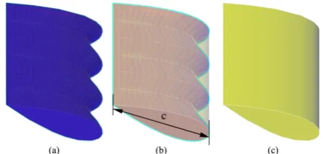
TLE amplitude was set to 0.02m and wavelength to 0.2m to keep the A/W ratio low at 0.1 or the amplitude at 10% of the wavelength. The wavelength is 4/3 of the chord. The 3D cambered TLE geometry was likewise treated as an infinitesimal blade unit with both of its ends terminating in the sinusoidal wave crests. Fig. 2 shows the isometric and orthographic views of the 3D TLE model where the resulting modified blade has three tubercles on the airfoil leading edge. Fig. 3 shows a comparative perspective of the 3D cambered and TLE blades. It showcases the former containing the latter to highlight their geometric differences.

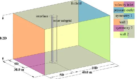
The simulation domain was discretized into the rotor sub-grid and stationary farfield sub-sub-grid compliant to the sliding mesh technique. The rotor sub-grid is a 4.2m-diameter cylinder containing the VAWT geometry with the center hub at the origin of the x-y-z Cartesian coordinate system. In fully developed flows, a significant extension of the fluid around the VAWT rotates with it. The rotor sub-grid is contained in a cylindrical opening in the farfield sub-grid dimensioned 30m in width and 40m in length, with the shorter sides to the left and right of the rotor, and the lengths up and below equidistant to the rotor. The farfield sub-grid extends up, below and left of the rotor 15m or five rotor

diameters away from the center hub, and to the right, 25m or 10 rotor diameters away. Both the rotor and farfield sub-grids are 0.2 rotor diameters or 0.6m thick.

Creating the 3D mesh involved initially making surface meshes on the domain boundaries and growing the volume mesh from these surface meshes inward. The discretized 3D domain in Fig. 4 details the boundary conditions of the farfield sub-grid. The farfield sub-grid mesh, set with a boundary decay of 0.95 and cell growth of 1.1, is coarse and fully unstructured but still hexahedral-dominant. The rotor sub-grid mesh is mixed-cell in nature. Meshes around the blades up to 90 cell layers are structured O-type meshes with Δs set to y+ _{= 0.1, after which the meshes grow outwards}

unstructured with boundary decay of 0.3 and cell growth of 1.1. Average cell size in the rotor sub-grid needs to be less than the c. Cell skewness was set to 0.6. This was monitored in the final mesh along with cell orthogonality and cell aspect ratio. Table 1 compares the cell populations of the 3D cambered and TLE VAWTs along with the 2D baseline. Cell size and distribution of the TLE VAWT rotor sub-grid are contrasted with the chord length in Fig. 5.

B. Steady Wind Simulation

The y+ _{and node density settings were established with the}

parametric studies conducted after the mesh and model validations done on a baseline 2D mesh equivalent of the 3D domain. The baseline 2D mesh with 210-node airfoils, y+

setting of 1 and time step equivalent to 1˚ azimuth was tested for numerical and statistical convergence, and mesh validity to validate the model and mesh, respectively. Simulation run resulted with statistical convergence noticeable at the fifth VAWT rotation and fully developed at the tenth and last rotation. Numerical convergence was also achieved with all conserved variables falling below the minimum of 1.0 x 10-6_.

y+ _{monitoring showed the blade-adjacent cells to have values}

oscillating within the range of 0 to 1 as needed to validate the mesh for the turbulence model. Parametric studies on the y+_{, node density and time step established the validity of the}

Fig. 3. Perspective views of the (a) TLE cambered blade, (b) TLE inside the straight cambered blade and the (c) straight cambered blade.

Fig. 2. (a) Isometric and (b-d) orthographic views of the cambered TLE blade geometry.

TABLEI

CELL POPULATION OF DISCRETIZED DOMAINS

Model Domain Cell Population

2D (baseline) Farfield sub-grid 2,769

Rotor sub-grid 59,865

3D (cambered) Farfield 21,253

Rotor 1,666,420

3D Farfield 21,253

(cambered

2D baseline mesh as the optimal among the test meshes. Rotor sub-grid rotation for each simulation was set to the constant ω based on the λ setting. Velocity inlet U was constant at 5 m/s for steady wind flow. Therefore, at the peak λ of 4, ω is 13.33 m/s and Re ≈ 2.0 × 105_{. k-ω SST}

turbulence model was used to solve the pressure-based, transient RANS equations. Model default settings were used with the Production Limiter option toggled on for turbulence energy correction in the ω equation.

Simulations required 10 complete rotor revolutions for the solution and residuals to converge. Interpolation schemes of pressure, momentum, turbulent kinetic energy and specific dissipation rate were all of second order with coupling set for the pressure and velocity components. Coefficients of lift, drag and moment on all three blades were individually monitored throughout the simulation.

Instantaneous torque was computed using (2). Net torque TB is the summation of all torque blades for an instance. The

instantaneous CP for each torque value was determined using

(3). The mean CP for one full rotation is taken as the average

of the last two VAWT rotations.

m Lc AV

T 2

2 1



 (2)

m

P c

C  (3)

The performance curves of the 2D and 3D models are shown in Fig. 6 alongside benchmark curves from literature [9],[16] where the CP results of the former show precise

agreement with the latter concluding the suitability as models and the validity of results of the 2D and 3D models. y+ _{values of near-blade cells in the 3D model have also been}

monitored to be within the target range of 0 to 1.

III. RESULTS AND DISCUSSION

Monitored torque values in Fig. 7 for one complete rotation of coincident blades for each of the cambered and TLE VAWTs show straightforward visual deviation of results between the two. Torque values plotted are for the tenth rotation of a single blade for each VAWT checked for numerical and cyclical convergence. While both blades follow the same torque curve path at the start, torque values of the TLE blade begin departing from the baseline at θ = 55°, therein labeled 1, when the cambered blade is still trailing linearly towards its peak T = 4.57Nm at θ = 90˚. Instead of sustaining or surpassing the peak torque of the cambered blade, the TLE blade had an earlier onset of torque reversal, which also means a shift in forces acting on it during the period.

Referring again to Fig. 7, during the period labeled 1 to 2 in the torque curve, both the cambered and TLE blades experience approximately the same drag forces shown as labeled in the plot of CD against AOA in Fig. 9. After θ =

74˚, labeled 3 in the torque curve, the TLE blade encounters dipping of its torque until values become negative due to drag forces overturning the net positive torque on the blade. From 3 up to the lowest point in the torque curve at θ = 106° labeled 4, the TLE blade encounters progressive linear decline in torque until it reaches the lowest or most negative value of -3.59Nm. For this period, CD behavior is inversely

-4.5 -3.5 -2.5 -1.5 -0.5 0.5 1.5 2.5 3.5 4.5 5.5

0° 30° 60° 90° 120°150°180°210°240°270°300°330°360°

T

o

rq

u

e

, T

(

N

·m

)

Azimuth, θ Straight TLE

1 2

3

4

5

Fig. 7. Individual blade torque curve comparison of cambered and TLE blades over one VAWT rotation

Fig. 5. (a) 3D domain of the mixed-cell rotor sub-grid with the structured O-mesh control cylinders flanked by unstructured hex-dominant cells and (b) zoom-in of the TLE blade and near-wall cells.

-0.10 0.00 0.10 0.20 0.30 0.40 0.50

0.0 1.0 2.0 3.0 4.0 5.0 6.0 7.0

P

o

w

e

r

c

o

e

ff

ic

ie

n

t,

CP

Tip Speed Ratio, λ

NACA 0025 (CMDMS) [16] NACA 0025 (CFD) [9] NACA 1425 (CFD) [9] 2D validation study Betz limit 3D validation study

increasing as depicted in the corresponding labels of Fig. 9, peaking approximately at the maximum negative torque. There is an observable delay of 5°, which can be hysteresis on resulting blade torques by the acting forces or force interactions. The CD for the TLE blade is thus observed to

peak 5° before the lowest torque at 4. Up to this rotation period, the only noted difference in the CL of the blades is

the advanced peaking and lower peak value for the TLE blade with the deviation beginning at the same azimuth of interest, θ = 55°. The TLE blade has peak CL = 0.80 at θ =

90° while the baseline has peak CL = 0.87 at θ = 96°.

Lowering the lift and increasing drag reversed the net moment on the blade.

After 4, the torque and lift of the TLE blade recover so that between the period of θ = 180° to 360°, labeled 5 to 1 in Fig. 7 to 9, the averages for the T, CL and CD are 0.49Nm,

-0.34 and 0.035, respectively. Except for the CD averaged at

0.042, the averages of T and CL for the cambered blade over

the same period are the same. This makes the period between θ = 0° to 180° the azimuth range of interest.

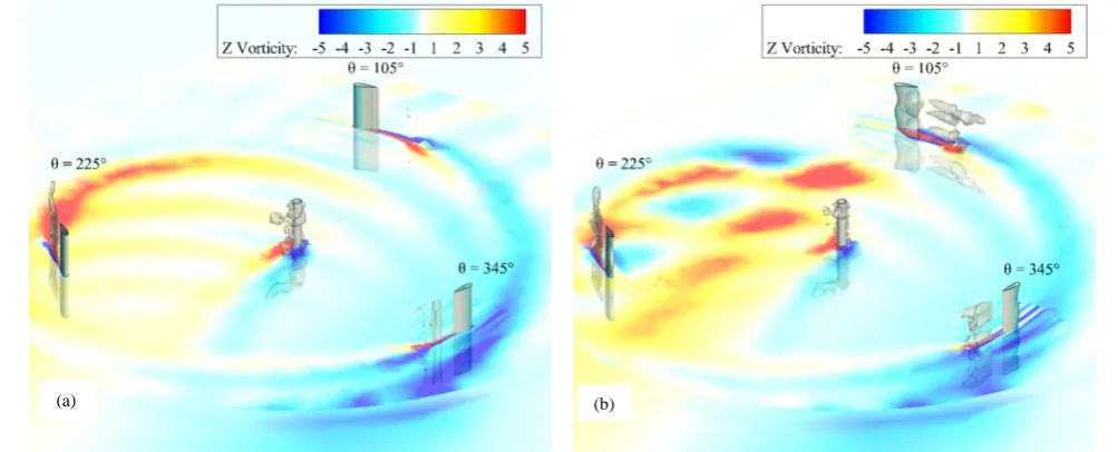
A vorticity profile of the fluid space surrounding the blades gives insight into the phenomena happening for the azimuth range of interest on the TLE blade. Comparing the vorticities of the cambered and TLE blades at θ = 105° in Fig. 11 shows a striking contrast of wind flow at the blade wakes. At the specified azimuth, the cambered blade vorticity profile shows streamlined flow instead of vortex

generation at the blade wake. The TLE blade, on the other hand, has explicitly massive vortices the size of the chord emanating from just before the trailing edge. It is at this time that the TLE blade experiences the maximum negative T and peak CD. Despite not shown, the same vortex profile of the

TLE blade proliferates until θ = 180°, therewith the large vortices have fully disintegrated and flow has become streamlined like that of the cambered blade. Thus, at the same vortical scales of Q-criterion, the TLE blade has been shown to generate vortices severely increasing the flow-induced drag and consequently reducing the blade torque.

Using the same vorticity plot of Fig. 11 shows remarkable similarity of blade wakes in both blade types at θ = 345° and 225°. This is expected as between θ = 180° to 360°, both blades have the same net torque and CL values.

Besides generating blade wake vortices, the TLE modification affects vortex shedding as depicted by the altered vortex street in the z-vorticity profile at mid-blade or z = 0. This reduces the T yet again at θ = 269° from Fig. 7.

Due to the large negative torque upwind of the TLE VAWT, its cycle-averaged torque is 0.24Nm. This is a quarter of the torque generated with the cambered blade. This value, though, amounts to no usable torque when the combined net blade torque of the three TLE blades superimpose values that yield a net negative for one full rotation.

Available PW for the VAWT totals 137.8W. The baseline

Fig. 11. Vorticity plot using z-vorticity slice at z = 0 and Q-criterion iso-surface for the (a) cambered VAWT and (b) TLE VAWT.

(a) _(b)

-0.8 -0.6 -0.4 -0.2 0 0.2 0.4 0.6 0.8 1

-16°-14°-12°-10° -8° -6° -4° -2° 0° 2° 4° 6° 8° 10° 12° 14° 16°

C

o

effi

ci

ent

o

f li

ft,

CL

Angle-of-attack, α Cambered

TLE

1

2 3

4

5

Fig. 8. CL vs. α plot.

0 0.03 0.06 0.09 0.12 0.15 0.18 0.21 0.24 0.27

-16°-14°-12°-10° -8° -6° -4° -2° 0° 2° 4° 6° 8° 10° 12° 14° 16°

C

o

effi

ci

ent

o

f drag

,

CD

Angle-of-attack, α Cambered

TLE

1

2 3

5

4

IV. SUMMARY AND CONCLUSION

Using torque, lift and drag data, the TLE modification on a cambered airfoil was shown to be detrimental to flow and performance. Analyses and observations were verified using the vorticity profiles of the steady wind flow simulations comparing the z-vorticity slice mid-blade and a Q-criterion iso-surface depicting flow vortices. Where the baseline cambered VAWT appeared to have streamlined flow generally throughout the steady wind flow, the TLE VAWT has been generating massive vortices at blade wakes at azimuthal positions between 106° to 180°. The TLE blades have deteriorated flow based on the negative torques from θ = 55° to 186°. A cambered VAWT blade experiences torque peak at the upwind leeward side when the blade has been in cross-flow with the steady wind stream but encounters flow degradation thereafter.

Based on a medley of researches, Aftab [13] claims the TLE to behave much like vortex generators. Indeed, the TLE in the VAWT has generated vortices very distinguishable in the Q-criterion vorticity profiles. Generated vortices however amounted to negative torque values up to -3.59Nm that degraded performance. A TLE blade in a VAWT generates turbulence instead of containing or decreasing it as was presumed. It also appears that at 120° angle of separation, a succeeding TLE blade encounters and is affected by the turbulence generated by the previous TLE blade. A three-bladed H-rotor Darrieus VAWT configuration may not allow ample time for the turbulent structures to dissipate and for a blade to recover from blade wake turbulence.

[3] W. A. Timmer and C. Bak, “Aerodynamic characteristics of wind turbine blade airfoils,” Advances in wind turbine blade design and materials, P. Brøndsted and R. P. L. Nijssen, Eds. Cambridge, UK: Woodhead Publishing Limited, 2013.

[4] SAS IP, Inc., ANSYS Fluent Theory Guide, USA, 2016.

[5] J. M. Edwards, L. A. Danao and R. J. Howell. (2012). Novel experimental power curve determination and computational methods for the performance analysis of vertical axis wind turbines. Journal of

Solar Energy Engineering. [Online]. Available: doi:

10.1115/1.4006196

[6] M. R. Castelli, et al, “Modeling Strategy and Numerical Validation for a Darrieus Vertical Axis Micro-Wind Turbine,” Proceedings of the ASME 2010 International Mechanical Engineering Congress &

Exposition IMECE 2010, ASME, 2010.

[7] S. N. Zadeh, M. Komeili and M. Paraschivoiu, “Mesh convergence study for 2-D straight-blade vertical axis wind turbine simulations and estimation for 3-D simulations,” Transactions of the Canadian Society for Mechanical Engineering, vol. 38, no. 4, pp. 487-504, Canadian Society for Mechanical Engineering, 2014.

[8] R. Bourguet, G. Martinat, G. Harran and M. Braza, Aerodynamic multi-Criteria shape optimization of VAWT blade profile by viscous approach,” Wind Energy: Proceedings of the Euromech Colloquium, J. Peinke, P. Schaumann and S. Barth, Eds., Berlin Heidelberg, Germany: Sprein Springer-Verlag, 2007.

[9] M. D. Bausas and L. A. M. Danao, “The aerodynamics of a camber-bladed vertical axis wind turbine in unsteady wind,” Energy, 93, pp. 1155-1164, 2015.

[10] V. Rolin and F. Porté-Agel, “Wind-tunnel study of the wake behind a vertical axis wind turbine in a boundary layer flow using stereoscopic particle image velocimetry,” Journal of Physics: Conference Series, 625, IOP Publishing, 2015.

[11] L. Battisti, A. Brighenti, E. Benini, M. R. Castelli, “Analysis of Different Blade Architectures on small VAWT Performance,”

Journal of Physics: Conference Series, 753, IOP Publishing, 2016.

[12] A. Loya, M. Z. U. Khan, R.A. Bhutta and M. Saeed, “Dependency of Torque on Aerofoilcamber Variation in Vertical Axis Wind Turbine,”

World Journal of Mechanics, 6, 472-486, 2016.

[13] S. M. A. Aftab et al, “Mimicking the humpback whale: An aerodynamic perspective,” Progress in Aerospace Sciences, 84, pp. 48-69 2016.

[14] F. E. Fish and J. M. Battle, “Hydrodynamic design of the humpback whale flipper,” Journal of Morphology, pp. 1-60, Wiley-Liss, Inc. , 1995.

[15] D. S. Miklosovic et al., “Leading-edge tubercles delay stall on humpback whale (Megaptera novaeangliae) flippers.” Physics of

Fluids, vol. 16 no. 5, pp. L39-L42, AIP, 2004.

[16] M. Wahl, Designing an H-rotor type Wind Turbine for Operation on

Amundsen-Scott South Pole Station, Published Master’s Thesis,

Uppsala University, Sweden, 2007.

[17] K. L. Hansen, Effect of Leading Edge Tubercle on Airfoil

Performance, PhD thesis, The University of Adelaide, Australia,

2012.

[18] H. T. C. Pedro and M. H. Kobayashi, “Numerical study of stall delay on humpback whale flippers,” 46th AIAA Aerospace Sciences

Meeting and Exhibit, 7-10 January 2008, Reno, Nevada, American

Institute of Aeronautics and Astronautics, Inc., 2008.

[19] Z. Wang and M. Zhuang. (2017). Leading-edge serrations for performance improvement on a vertical-axis wind turbine at low tip-speed-ratios. Applied Energy [Online]. vol. 208, pp. 1184-1197. Available: http://dx.doi.org/10.1016/j.apenergy.2017.09.034 [20] C.-J. Bai, Lin, Y.-Y., Lin, S.-Y. and W.-C. Wang, “Computational

fluid dynamics analysis of the vertical axis wind turbine blade with tubercle leading edge,” Journal of Renewable Sustainable Energy, 7 (3), AIP, 2015.

[21] A. Corsini and G. Delibra, “On the Role of Leading-Edge Bumps in the Control of Stall Onset in Axial Fan Blades,” Journal of Fluids

Engineering, 135, pp. 081104, ASME, 2013.

NOMENCLATURE

Symbol Quantity/Definition Units

y+ _{dimensionless wall distance -}

Δs wall spacing m

θ azimuth °

α angle-of-attack ˚

V wind velocity m/s

Vb blade velocity m/s

ω rotational velocity rad/s

R rotor m

T blade torque Nm

ρ density kg/m3

A area m2

L characteristic length m

λ tip speed ratio dimensionless

Re Reynolds number dimensionless

Cm moment coefficient dimensionless

CL lift coefficient dimensionless

CD drag coefficient dimensionless

PW wind power W

A amplitude m

W wavelength m

A/W amplitude to wavelength ratio dimensionless

NACA National Advisory Committee

for Aeronautics

-