Poisson-Fermi modeling of ion activities in aqueous single and mixed electrolyte solutions at variable temperature

Poisson-Fermi modeling of ion activities in aqueous single and mixed electrolyte

solutions at variable temperature

Jinn-Liang Liu, and Bob Eisenberg

Citation: The Journal of Chemical Physics 148, 054501 (2018);

View online: https://doi.org/10.1063/1.5021508

View Table of Contents: http://aip.scitation.org/toc/jcp/148/5

Poisson-Fermi modeling of ion activities in aqueous single

and mixed electrolyte solutions at variable temperature

Jinn-Liang Liu1,a)_{and Bob Eisenberg}2,b)

1_{Institute of Computational and Modeling Science, National Tsing Hua University, Hsinchu 300, Taiwan} 2_{Department of Physiology and Biophysics, Rush University, Chicago, Illinois 60612, USA and Department}

of Applied Mathematics, Illinois Institute of Technology, Chicago, Illinois 60616, USA

(Received 4 January 2018; accepted 13 January 2018; published online 1 February 2018)

The combinatorial explosion of empirical parameters in tens of thousands presents a tremendous chal-lenge for extended Debye-H¨uckel models to calculate activity coefficients of aqueous mixtures of the most important salts in chemistry. The explosion of parameters originates from the phenomenologi-cal extension of the Debye-H¨uckel theory that does not take steric and correlation effects of ions and water into account. By contrast, the Poisson-Fermi theory developed in recent years treats ions and water molecules as nonuniform hard spheres of any size with interstitial voids and includes ion-water and ion-ion correlations. We present a Poisson-Fermi model and numerical methods for calculating the individual or mean activity coefficient of electrolyte solutions with any arbitrary number of ionic species in a large range of salt concentrations and temperatures. For each activity-concentration curve, we show that the Poisson-Fermi model requires only three unchanging parameters at most to well fit the corresponding experimental data. The three parameters are associated with the Born radius of the solvation energy of an ion in electrolyte solution that changes with salt concentrations in a highly nonlinear manner.Published by AIP Publishing.https://doi.org/10.1063/1.5021508

I. INTRODUCTION

Thermodynamic modeling of aqueous electrolyte solu-tions plays an important role in chemical and biological sci-ences.1–13 _{Despite intense efforts in the past century, robust}

thermodynamic modeling of electrolyte solutions still presents a difficult challenge and remains a remote ambition in the extended Debye-H¨uckel (DH) models due to the enormous number of parameters that need to be adjusted, carefully and often subjectively.11,13 For example, the Pitzer model requires 8 parameters for a ternary system and up to 8 tem-perature coefficients (parameters) for every Pitzer parameter in a temperature interval from 0 to about 200 ◦C.11,13 It is indeed a frustrating despair (frustration on p. 11 in Ref. 9

anddespairon p. 301 in Ref. 1) that approximately 22 000 parameters for combinatorial solutions of the most important 28 cations and 16 anions in salt chemistry have to be extracted from the available experimental data for one temperature.11

The Pitzer model is still the most widely used DH model with unmatched precision for modeling aqueous electrolyte solutions over wide ranges of composition, temperature, and pressure.13

The Pitzer model and its variants13are all derived from the Debye-H¨uckel theory14 that in turn is based on a lin-ear Poisson-Boltzmann (PB) equation5 although potentials calculated from PB near ions (for example) are often far beyond the linear range of the potential near ions or inter-faces. The PB equation treats ions as point charges with-out steric volumes and water molecules as a homogeneous

a)_{Author to whom correspondence should be addressed: [email protected]} b)_{E-mail: [email protected]}

dielectric medium without steric volumes either and with a constant dielectric constant that neglects ion-water and ion-ion correlations. These simplifications give rise to the elegant, sim-ple, and useful DH theory. However, it is precisely because of the linearization and simplifications on steric and correlation effects that extended DH models have needed an explosion in the number of parameters in order to overcome the defi-ciencies (simplifications) of the classical Poisson-Boltzmann theory. The nonlinear PB equation was developed by Gouy and Chapman.15,16

In the past few years, we have intensively investigated these two effects in a range of areas from electric dou-ble layers17,18 and ion activities19 to biological ion chan-nels18,20–24and consequently developed an advanced theory— the Poisson-Fermi (PF) theory—that treats ions and water molecules as nonuniform hard spheres of any size with inter-stitial voids and includes many of the correlation effects of ions and water. We refer to our previous papers and refer-ences therein for a historical account of the literature of this theory. In Ref. 19, we proposed a PF model for calculating activity coefficients of individual ions in aqueous single NaCl and CaCl2electrolyte solutions at the temperature 298.15 K.

The model is further tested in this paper for eight 1:1 elec-trolytes (LiCl, LiBr, NaF, NaCl, NaBr, KF, KCl, and KBr), six 2:1 electrolytes (MgCl2, MgBr2, CaCl2, CaBr2, BaCl2,

and BaBr2), one mixed electrolyte (NaCl + MgCl2), one 1:1

electrolyte (NaCl) at various temperatures from 298.15 to 573.15 K, and one 2:1 electrolyte (MgCl2) at various

tempera-tures from 298.15 to 523.15 K, for which the experimental data were compiled by Valisk´o and Boda in Ref. 25 and Rowlandet al.in Ref.13from various experimental sources in Refs.26–35.

054501-2 J.-L. Liu and B. Eisenberg J. Chem. Phys.148_{, 054501 (2018)}

The PF model is developed to calculate individual ion activities for which experimental measurements and determi-nation,10,36,37_{interpretation of measurement data,}26,37–39_and

comparison of different experimental methods37,40_{have been}

extensively investigated by Wilczek-Vera, Rodil, and Vera in the past two decades. PF results on mean activity coefficients can be compared with experimental measurements using the Debye-H¨uckel equation of individual ion activities.5

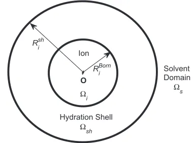
In contrast to the Pitzer model, we show that all exper-imental data sets of individual or mean activity coefficients as a function of variable concentration in single electrolytes or mixtures at various temperatures can be well fitted by the PF model with only 3 parameters at most for each activity-concentration data curve. The model is characterized by three different domains, namely, the Born ion, hydration shell, and remaining solvent domains in which the Born ion domain is most crucial because all activities around an ion are mainly governed by the singular charge of the ion located at the cen-ter of the domain. The Born ion domain is defined by the Born radius of the solvated ion, which is unknown and changes with salt concentrations in a highly nonlinear manner.

The three parameters characterize three orders of approx-imation of the Born radius in terms of ionic concentrations. Parameter 1 describes a correction of the experimental Born radius of a single ion in pure water without any other ions. Parameter 2 describes an adjustment of the unknown Born radius in electrolyte solution that accounts for the Debye screening effect, which is proportional to the square root of the ionic strength of the solution. Parameter 3 is an adjust-ment in the next order approximation beyond the DH treatadjust-ment of ionic atmosphere. The physical origin of these param-eters is clear unlike that of most paramparam-eters in the Pitzer method.11,41_{It may even be possible in later work to calculate}

some of these parameters from more detailed versions of our model.

Our approach to partition the free energy domain of a solvated ion into the above three sub-domains yields a better approximation to calculate the free energy since these sub-domains are determined by the experimental data of solvation and thus separate short- and long-range interactions of the ion in a more accurate way. This approach nevertheless incurs more complicated numerical methods for solving the nonlin-ear partial differential equations of the PF model in different domains with suitable interface conditions.17 We therefore present numerical methods in detail for future verification and development of the present work.

II. THEORY

For an aqueous electrolyte solution withKspecies of ions, the Poisson-Fermi theory proposed in Refs.18and21treats all ions and water of any diameter as nonuniform hard spheres with interstitial voids between these spheres. The activity coef-ficient γi of an ion of speciesiin the solution describes the

deviation of the chemical potential of the ion from ideality (γi

= 1). The excess chemical potential µex_i = kBTlnγi can be

calculated by19,42

µex

i =∆Gi−∆G0i, ∆Gi=

1

2qiφ(0), ∆G

0

i =

1 2qiφ

[image:3.594.331.521.49.190.2]

0_{(0), (1)}

FIG. 1. The model domainΩis partitioned into the ion domainΩi(with radius

R_iBorn), the hydration shell domainΩsh(with radiusRshi ), and the remaining

solvent domainΩs.

wherekBis the Boltzmann constant,T is an absolute

temper-ature,qiis the ionic charge of the hydrated ion (also denoted

byi),φ(r) is a potential function of spatial variable rin the domainΩ=Ωi∪Ωsh∪Ωsshown in Fig.1,Ωiis the spherical

domain occupied by the ioni,Ωshis the hydration shell domain

of the ion,Ω_sis the remaining solvent domain,0denotes the center (set to the origin) of the ion,φ(0) is the value ofφ(r) at r=0, andφ0(r) is a potential function when the solvent domain Ω_s does not contain any ion at all with pure water only. The potential functionφ(r) can be found by solving the Poisson-Fermi equation18

l_c2∇2−1∇ ·(r)∇φ(r)=ρ(r), (2)

(r)=  



s=w0inΩsh∪Ωs

i=ion0inΩi

,lc=    



2ajinΩsh∪Ωs

0 inΩi

,

(3)

ρ(r)=

         



ρs(r)=PKk=1qkCk(r) inΩs

0 inΩsh

ρi(r)=qiδ(r−0) inΩi

, (4)

Ck(r)=C_kBexp −βkφ(r) +

vk

v0

Strc(r)

!

inΩ, (5)

Strc(r)=ln Γ(r) ΓB

!

inΩ, (6)

where0 is the vacuum permittivity,wis the dielectric

con-stant of bulk water,ionis a dielectric constant inΩi,ajis the

radius of a counterion of the ioni, and δ(r 0) is the delta function at the origin.

The concentration functionCk(r) is described by a Fermi

distribution(5), whereCB

k is a constant bulk concentration for

allk = 1,. . .,K + 1,qK+1= 0, βk =qk/kBT,vk = 4πa_k3/3,

v0 =

_PK+1 k=1 vk

/(K + 1) an average volume of all kinds of hard spheres, Strc_{(r) is called the steric potential, Γ}B _{= 1}

−PK+1

k=1 vkCBk is a constant void fraction, Γ(r) = 1 − PK+1

k=1

vkCk(r) is a void fraction function, andK + 1 denotes water.

The radii ofΩiand the outer boundary ofΩshare denoted by

RBorn_i andRsh_i , respectively, whose values will be determined by experimental data. It is natural to choose the Born radius RBorn_i (not the ionic radiusai) as the radius ofΩi.42We consider

The potential φ0(r) [in Eq. (1)] of the ideal system is obtained by settingρs(r) = 0 in(4), i.e., all particles inΩsdo not

electrostatically interact with each other sinceqk= 0 for allk.

The domainΩis chosen to be sufficiently large so thatφ(r) = 0 on the boundary of the domain∂Ω. The ideal potentialφ0_(r)

is then a constant, i.e.,∆G0

i is a constant reference chemical

potential independent ofC_kB.

The distribution(5)is of Fermi type since all concentration functions have an upper bound, i.e.,Ck(r)<1/vkfor all particle

species with any arbitrary (or even infinite) potentialφ(r) at any locationrin the domainΩ.21The Poisson-Fermi equation(2)

and the Fermi distribution(5)reduce to the Poisson-Boltzmann equation and the Boltzmann distribution whenlc =Strc = 0,

i.e., when the correlation and steric effects are not considered. The Boltzmann distributionCk(r)=C_kBexp (−βkφ(r)) would

however diverge ifφ(r) tends to infinity. This is a major defi-ciency of the PB theory for modeling a system with strong local electric fields or interactions.45If the correlation lengthlc,0,

the dielectric operatorD=s(1−l

2

c∇2) in Eq.(2)approximates

the permittivity of the bulk solvent and the linear response of correlated ions17,20,46,47and yields a dielectric functionH(r) as

an output of solving Eq.(2).21The exact value ofH(r) at any

r∈Ω_sh∪Ω_scannot be obtained from Eq.(2)but can be approx-imated by the simple formulaH(r)≈i+CH2O(r)(s−i)/C

B H2O

since the water density function CH2O(r) = CK+1(r) is an

output of Eq.(5). This formula is only for visualizing (approxi-mately) the profile ofDorH. It is not an input of calculation. The

input is the correlation lengthlcin Eq.(3).17,20,46,47The actual

outputs are the numerical solutions of the partial differential equations and boundary conditions.

The factorvk/v0multiplying the steric potential function

Strc_{(r) in Eq. (5) is a modification of the unity used in our}

previous work.19,21The steric energy−vk v0S

trc_(r)k

BT21,24of a

typek particle depends not only on the voidness (Γ(r)) (or equivalently crowding) atrbut also on the volumevk of the

particle itself. If allvkare equal (and thusvk=v0), then all

par-ticle species at any locationr∈Ω_sh∪Ω_shave the same steric energy, i.e., uniform particles are indistinguishable in steric energy. The steric potential is a mean-field approximation of Lennard-Jones (L-J) potentials that describe local variations of L-J distances (and thus empty voids) between any pair of particles. L-J potentials are highly oscillatory and extremely expensive and unstable to compute numerically.21

Calcula-tions that involve L-J potentials or even truncated versions of L-J potentials must be extensively checked to be sure that results do not depend on irrelevant parameters.

III. METHODS

To avoid large errors in approximation caused by the delta function δ(r 0) in(4), the potential function can be decomposed as17,48,49

φ(r)= 



 H

φ(r) +φ∗(r) +φL(r) inΩ_i

H

φ(r) inΩ_sh∪Ω_s , (7)

whereφ∗(r)=qi/(4πi|r−0|) andφH(r) is found by solving

l_c2∇2−1∇ ·_s∇φH(r)=ρ(r) inΩsh∪Ωs, (8)

−∇ ·_i∇φH(r)=0 inΩ_i (9)

without the singular source term ρi(r) =qiδ(r0) and with

the interface conditions

       f H

φ(r)g =0

f

(r)∇φH(r)·n g

=i∇

φ∗

(r) +φL(r))·n for all

r∈∂Ω_i,

(10)

wherenis an outward normal unit vector atr∈∂Ω_iand the jump function [u(r)]=limrsh→ru(rsh)−limri→ru(ri) withrsh ∈Ω_shandri∈Ωi.17The potential functionφL(r) is the solution

of the Laplace equation

∇2φL(r)=0 inΩ_i (11)

with the boundary condition

φL

(r)=φ∗(r) on∂Ω_i. (12)

The evaluation of Green’s functionφ∗(r) on∂Ω_ialways yields finite numbers and thus avoids the singularity in the solution process. The desired solvation energy∆Giin Eq.(1)(and thus

the individual ionic activity coefficientγi) is then evaluated

by17,49

∆Gi=kBTlnγi=

1 2qi

f

H

φ(0) +φL(0)g. (13)

Since the interface∂Ω_iis a sphere centered at the origin, the Laplace potentialφL(r)=qi/(4πiR_iBorn) is a constant inΩi,

i.e., Eq.(11)has been exactly solved.

The Poisson-Fermi equation (8) is a nonlinear fourth-order partial differential equation (PDE) inΩ_s. Newton’s iter-ative method is usually used for solving nonlinear problems. We seek a sequence of approximate solutions(φHm(r)

)M

m=1by

iteratively solving the linearized PF equation

l2_c∇2−1∇ ·∇φHm−ρ0s(φHm−1)φHm

=ρs(φH_m−1)−ρ0s(φH_m−1)φH_m−1inΩs, (14)

until a tolerable potential function φHM is reached, where

H

φ0(r) is a given initial guess potential function, ρs(φHm−1)

=PK k=1qkCm

−1

k (r),C m−1

k (r)=C

B

k exp

−βkφHm−1(r) +v_vk₀S_mtrc₋₁

(r),S_mtrc₋₁(r) = lnΓ0(r) ΓB

, Γ_m−1(r) = 1−PK_k=+1₁ vkC_km−1(r),

ρ0

s(φHm−1) = PK_k=1(−βkqk)Cm_k−1(r), and ρ0s(φH) = d dφH

ρs(φH).

Note that the differentiation in ρ0s(φH) is performed only with

respect to φH, whereas Strc is treated as another

indepen-dent variable althoughStrcdepends onφHas well. Therefore,

ρ0

s(φH) is not exact implying that this is an inexact Newton’s

method.50

The fourth-order problem can be resolved by transforming Eq.(14)into two second-order PDEs17

s

l_c2∇2−1Ψ(r)=ρ(φHm−1) inΩsh∪Ωs, (15)

−_s∇2φHm(r)−ρ0(φHm−1)φHm(r)

= −_sΨ(r)−ρ0(φHm−1)φHm−1inΩsh∪Ωs (16)

by introducing a density like variableΨ=∇2φHfor which the

boundary condition is17

054501-4 J.-L. Liu and B. Eisenberg J. Chem. Phys.148_{, 054501 (2018)}

Equations(9),(15), and(16)are coupled together in the entire domainΩwith the jump conditions in(10). Note that linear PDEs(14)–(16)converge to the nonlinear PDE(8)ifφHM

con-verges to the exact solutionφHof Eq.(8)asM → ∞, i.e., the

approximate potentialφHM(r) is sufficiently close to the exact

potentialφH(r) for allr∈Ωsh∪Ωsif the iteration numberMis

sufficiently large (M≈5–37 for this work with error tolerance 103_).

The standard 7-point finite difference (FD) method is used to discretize all PDEs(9),(15), and(16), where the jump con-ditions in(10)are handled by the simplified matched interface and boundary (SMIB) method proposed in Ref.17. For sim-plicity, the SMIB method is illustrated by the following 1D linear Poisson equation (inx-axis):

−d

dx

"

(x)d dxφH(x)

#

=f(x) inΩ (18)

with the jump condition

f

φH

0g

=−_i d

dxφ ∗

(x) atx=ξ=∂Ω_i∩∂Ω_s, (19)

whereΩ=Ωi∪Ωs,Ωi= (0,ξ),Ωs= (ξ,L),f(x) = 0 inΩi,

f(x),0 inΩs, andφH

0 ₌ d

dxφH(x). The corresponding cases to

Eqs.(9),(15), and(16)in they- andz-axis follow in a similar way. Let two FD grid pointsxl andxl+1across the interface

pointξbe such thatxl < ξ <xl+1andξ= (xl+xl+1)/2 with

∆x=xl+1xl = 1 Å, a uniform mesh, for example, as used

in this work. The FD equations of the SMIB method atxland

xl+1are

i

−φHl−1+ (2−c1)φHl−c2φHl+1

∆x2 =fl+

c0

∆x2, (20)

s

−d1φHl+ (2−d2)φHl+1−φHl+2

∆x2 =fl+1+

d0

∆x2, (21)

where

c1=

i−s

i+s

,c2=

2s

i+s

,c0 =

−_i∆xfφH0 g

i+s

,

d₁= 2i i+s

,d₂= s−i i+s

,d₀=

−_s∆xfφH0 g

i+s

,

H

φl is an approximation ofφH(xl), andfl=f(xl). Note that the

jump valuefφH0 g

atξis calculated exactly since the derivative ofφ∗is given analytically.

Since the steric potential takes particle volumes and voids into account, the shell volumeVshof the shell domainΩshcan

be determined by Eqs.(5)and(6)as

Strc_sh = v0 vw

ln*

,

Ow_i

VshCB_K+1 +

-=ln Vsh−vwO

w

i

VshΓB !

, (22)

where the occupancy (coordination) numberOw

i is given by

experimental data.43,44_{The shell radiusR}sh

i ofΩshis thus

deter-mined. Note that the shell volume depends not only onOw

i but

also on the bulk void fractionΓB, namely,on all salt and water concentrations(CB_k).

[image:5.594.306.550.60.234.2]

As discussed in Ref. 25, the solvation free energy of an ion i should vary with salt concentrations and can be expressed by a dielectric constant (C_iB) that depends on

TABLE I. Values of model notations.

Symbol Meaning Value Unit

kB Boltzmann constant 1.38×1023 J/K

T Temperature TableII K

e Proton charge 1.602×1019 _C 0 Permittivity of vacuum 8.85×1014 F/cm ion,w Dielectric constants 1, TableII

lc= 2aj Correlation length j= Cl, etc. Å

Ow_i In Eq.(22) 1843,44

aLi+,a_Na+,a_K+ Radii 0.6, 0.95, 1.33 Å

a_Mg2+,a_Ca2+,a_Ba2+ Radii 0.65, 0.99, 1.35 Å

aF−,aCl−,aBr−,aH2O Radii 1.36, 1.81, 1.95, 1.4 Å

R0 Li+,R

0 Na+,R

0

K+ Born radii in Eq.(24) 1.3, 1.618, 1.95 Å

R0 Mg2+,R

0 Ca2+,R

0

Ba2+ Born radii 1.424, 1.708, 2.03 Å

R_F0−,R0_Cl−,R0_Br−, Born radii 1.6, 2.266, 2.47 Å

the bulk concentration C_iB of the ion. Therefore, the Born energy

∆GBorn_i = 1 w

−1

! _q2

i

8π0R0_i

(23)

with the Born radius R0_i in pure water should be modified with the concentration-dependent dielectric constant (C_iB). Equivalently, the Born radius in electrolyte solutions can be modified fromR0

i by a simple formula

RBorn_i (C_iB)=θ(C_iB)R0_i,

θ(C_iB)=αi₁+αi₂

CB_i

1/2

+αi₃

CB_i

3/2

, (24)

whereCB_i =C_iB/M is a dimensionless bulk concentration of type i ions, M is the molar concentration unit, and αi₁, αi₂, and αi₃ are adjustable parameters for modifying the exper-imental Born radius R0_i to fit experimental activity coeffi-cientsγithat change with the bulk concentration conditions

CB

i of the ion. The Born radii R0i in TableI are cited from

Ref.25, which are computed from the experimental hydration Helmholtz free energies of these ions given in Ref.6. Numer-ical values in Tables I and II are all experimental data for which their values are kept fixed throughout calculations once chosen.

The three parameters in Eq.(24)have physical or mathe-matical meaning unlike many parameters in the Pitzer model.41 Any model or numerical method incurs errors to approxi-mate a real system, i.e., it is impossible to obtain real Born radiusRBorn_i (CB_i) exactly. The first parameterαi₁is an adjust-ment of the experiadjust-mental Born radius R0_i when C_iB = 0 for all i. The second parameter αi

2 is an adjustment of

RBorn_i (C_iB) that accounts for the real thickness of the ionic atmosphere (Debye length), which is proportional to the square root of the ionic strength

√

Iin the Debye-H¨uckel the-ory.5 The third parameter αi₃ is simply an adjustment in the

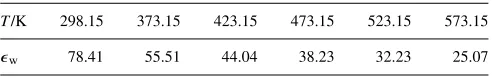
TABLE II. Values ofwat variousT.51

T/K 298.15 373.15 423.15 473.15 523.15 573.15

[image:5.594.306.552.709.748.2]

next order approximation beyond the DH treatment of ionic atmosphere.

We summarize the mathematical solution process for determining the activity of ionic solutions in the following algorithm.

1. Solve Eqs.(9),(10), and(16)for φHwithρ0=Ψ= 0 (in

pure water),RBorn_i =R0

i, andφL=qi/(4πiR0i) to obtain

∆G0_i by Eq.(13)and then setφH₀ =φH.

2. Solve Eqs.(15)and(17)forΨwithRBorn i in(24).

3. Solve Eqs. (9), (10), and (16) for φHm with φL =qi/(4πiRBorn_i ) and then setφHm−1 =φHm. Go to 2 until

convergence.

4. Obtain the activity coefficientγiby Eq.(13).

IV. RESULTS

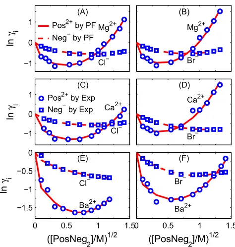
The PF results of ionic activity coefficients for eight 1:1 electrolytes, six 2:1 electrolytes, one mixed electrolyte, one 1:1 electrolyte at various temperatures, and one 2:1 electrolyte at various temperatures agree with the experimental data26–35as shown in Figs. 2–6, respectively. The empirical parameters used to fit the experimental data areαi₁,αi₂, andαi₃in Eq.(24), whose values are given in TableIIIfrom which we observe that the PF model requires only one to three parameters to fit those data.

The mean activity coefficientγPosNegof a salt PospNegq

is calculated via the formula lnγPosNeg = _pp_+qlnγPos

+_pq_+qlnγNeg,5whereγPosandγNegare individual activity

coef-ficients obtained by Eq.(13)for eachi=PosandNeg. For the mean activity coefficients of either ternary (Fig.4) or binary (Figs.5and6) systems, we only need to adjust 3 parameters of one cation (not all ions) as shown in TableIII.

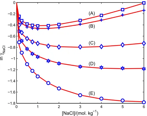
[image:6.594.309.546.44.293.2]

The activity coefficients by the PF model are quite suc-cessful over a large range of temperatures and concentrations as shown in Figs.4–6. We used the code of the density model

FIG. 3. Individual activity coefficients of 2:1 electrolytes. Comparison of PF results with experimental data26_{oni= Pos}2+_{(cation) and Neg(anion) activity}

coefficientsγiin various [PosNeg2] from 0 to 1.5M.

developed by Mao and Duan52 _{to convert the concentration}

unit from molality (mol Kg1_{) to molarity (M = mol dm}3₎

by the standard formula as given in Ref.52, where the den-sity model has been compared with thousands of measure-ments at high accuracy. The pressure values needed in the code at the corresponding temperatures were set to P = (a) 1.01, (b) 1.01, (c) 15.48, (d) 39.59, and (e) 80.50 bars for Fig.5and (a) 1.01, (b) 1.01, (c) 4.73, and (d) 39.50 bars for Fig.6. In Fig.4, the ionic strengthI =P

iCBiz

2

i and the ionic

strength fraction yMgCl2 = 3mMgCl2/(3mMgCl2 +mNaCl) with

mMgCl2 andmNaCl being the molalities of MgCl2 and NaCl

FIG. 2. Individual activity coefficients of 1:1 electrolytes. Comparison of PF results with experimental data26 _{on i}

= Pos+_{(cation) and Neg(anion)}

[image:6.594.44.382.498.753.2]

[image:7.594.49.288.47.238.2]

054501-6 J.-L. Liu and B. Eisenberg J. Chem. Phys.148_{, 054501 (2018)}

FIG. 4. Mean activity coefficients of mixed electrolytes. Comparison of PF results (curve) with experimental data (symbols) compiled in Ref.13(a) from Ref.33on mean activity coefficientsγof NaCl as a function of the ionic strength (I) fractionyMgCl2of MgCl2in NaCl + MgCl2mixtures atI= 6 mol

Kg1andT= 298.15 K and (b) from Ref.34(circles) and Ref.35(squares) onγof NaCl as a function of the MgCl2molality in NaCl + MgCl2mixtures

at [NaCl] = 6 mol Kg1andT= 298.15 K.

in the mixture, respectively, whereziis the valence of typei

ions.

We observe from TableIIIthat the approximateRBorn i (CBi)

(with salts) deviates fromR0_i (without salts) only in the second to fourth decimal place, i.e., numerical values ofγiare very

sensitive to the decimal order ofαi₁,αi₂, andαi₃ because the Born radiusRBorn_i (C_iB) is very close to the origin0at which the singular charge in ρi(r) =qiδ(r0) is infinite. The

approxi-mation of the shell radiusRSh_i [or the coordination numberOw_i in Eq.(22)], on the other hand, is much less significant than that ofRBorn

i because the electric potentialφPF(r) diminishes

[image:7.594.310.548.48.236.2]

exponentially in the hydration shell regionΩshas shown by

FIG. 5. Mean activity coefficients of 1:1 electrolyte at various temperatures. Comparison of PF results (curves) with experimental data (symbols) compiled in Ref.13from Refs.27–29on mean activity coefficientsγof NaCl in [NaCl] from 0 to 6 mol Kg1_{atT= (a) 298.15, (b) 373.15, (c) 473.15, (d) 523.15,}

(e) 573.15 K.

FIG. 6. Mean activity coefficients of 2:1 electrolyte at various temperatures. Comparison of PF results (curves) with experimental data (symbols) compiled in Ref.13from Refs.30–32on mean activity coefficientsγof MgCl2in

[MgCl2] from 0 to 6 mol Kg1atT= (a) 298.15, (b) 373.15, (c) 423.15, (d)

523.15 K.

the profile ofφPF(r) in Fig.7. The values ofαi₁,αi₂, andαi₃ for each activity-concentration curve were obtained by first tuning three values of θ(C_iB) in Eq.(24)to match three data

points (qCB

ij, lnγij) with three different concentrationsCijB,j

= 1, 2, 3, and then solving the three unknownsαi₁,αi₂, andαi₃ using three knownθ(CB

ij) values. For example, for thei= Li+

curve in Fig.2(a), the selected experimental data points are (qC_ijB, lnγij) = (0.315,0.192), (1,0.007), and (1.577, 0.57)

and the corresponding tuned θ(CB

ij) are 0.9996, 1.0013, and

1.0043.

The PF model can provide more physical details near the solvated ion (Ca2+, for example) in a strong electrolyte ([CaCl2] = 2M) such as (1) the dielectric functionH(r) with

its varying permittivity, (2) variable water density CH2O(r),

(3) concentration of counterionC_Cl−(r), (4) electric potential

φPF_{(r), and (5) the steric potentialS}trc_{(r) all shown in Fig.7.}

The steric potential is small because the configuration of par-ticles (voids between parpar-ticles) does not vary too much from the solvated region to the bulk region. Nevertheless, it has sig-nificant effect on the variation of mean-field water densities CH2O(r) and hence on the dielectric functionH(r) in the

hydra-tion region. Note thatH(r) is an output, not an input of the

model.

The strong electric potential φPF_{(r) in the Born}

cav-ity Ωi (with RBorn_i (C_iB) = 1.7130 Å) and the water density

CH2O(r) in the hydration shellΩsh (withR

sh

Ca2+ = 5.0769 Å)

are the most important factors allowing the PF results to match the experimental data. The ion and shell domains are the crucial region to study ion activities. For exam-ple, Fraenkel’s theory is entirely based on this region—the so-called smaller-ion shell region.41 The steric energy of water molecules modified by the factor vK+1/v0 in Eq. (5)

leads to significant changes ofCH2O(r) andH(r) profiles in

[image:7.594.48.287.508.696.2]

TABLE III. Values ofα₁i,α₂i, andαi₃in Eq.(24).

Figures i αi

1 α

i

2 α

i

3 Figures i α i

1 α

i

2 α

i 3

2(a) Li+ _{0.999 13 0.000 69 0.000 09 3(c) Ca}2+ _{0.998 86 0.000 46 0.000 11}

2(a) Cl 0.998 93 0.000 08 3(c) Cl 0.998 77 0.000 60 0.000 12 2(b) Li+ _{0.999 58 0.000 19 0.000 15 3(d) Ca}2+ _{0.998 86 0.000 99 0.000 17}

2(b) Br 0.998 22 0.001 07 3(d) Br 0.999 20 0.001 98 0.000 16 2(c) Na+ _{0.999 10 3(e) Ba}2+ _{0.998 44 0.000 11 0.000 10}

2(c) F 0.999 33 0.000 29 3(e) Cl 0.998 87 0.000 58 0.000 01 2(d) Na+ 0.999 27 0.000 26 0.000 04 3(f) Ba2+ 0.998 51 0.000 54 0.000 08 2(d) Cl 0.998 40 3(f) Br 0.999 26 0.001 45 0.000 18 2(e) Na+ 0.999 62 0.000 38 0.000 10 4(a) Na+ 1.005 81 0.000 13

2(e) Br 0.998 70 0.000 17 0.000 04 4(b) Na+ _{1.005 27 0.000 42 0.000 19}

2(f) K+ 0.999 34 0.001 20 0.000 07 5(a) Na+ 0.998 1 0.000 1 2(f) F 0.999 04 0.000 13 0.000 04 5(b) Na+ _{0.997 1 0.000 3 0.000 1}

2(g) K+ 0.999 29 0.001 22 0.000 04 5(c) Na+ 0.994 5 0.000 7 0.000 1 2(g) Cl 0.998 97 0.000 12 0.000 03 5(d) Na+ 0.992 5 0.002 8 0.000 1 2(h) K+ _{0.999 31 0.000 13 5(e) Na}+ _{0.987 0 0.004 2 0.001 0}

2(h) Br 0.999 45 0.001 75 0.000 06 6(a) Mg2+ 0.998 8 0.000 2 0.000 2 3(a) Mg2+ _{0.999 18 0.000 44 0.000 11 6(b) Mg}2+ _{0.998 9 0.000 4 0.000 3}

3(a) Cl 0.998 93 0.000 51 0.000 10 6(c) Mg2+ 0.998 3 0.001 4 0.000 5 3(b) Mg2+ _{0.999 10 0.00063 0.000 15 6(d) Mg}2+ _{0.996 1 0.002 0 0.000 3}

3(b) Br 0.998 88 0.000 65 0.000 18

Default values:αi 1=1,α

i

2=0, andα i 3=0.

FIG. 7. Dielectric functionH(r) (denoted byεin the

fig-ure), water densityCH2O(r) (CH2O), Clconcentration

CCl−(r) ([Cl]), electric potentialφPF(r) (φ), and steric

potentialStrc_{(r) (S}trc_{) profiles near the solvated ion Ca}2+

at [CaCl2] = 2M, whereris the distance from the center

of Ca2+in angstrom.

V. CONCLUSION

A Poisson-Fermi model for calculating activity coeffi-cients of aqueous single or mixed electrolyte solutions in a large range of concentrations and temperatures has been pre-sented and tested by a set of experimental data. The model was shown to well fit experimental data with only three adjustable parameters at most for each activity-concentration curve. The adjustable parameters correspond to different orders of approximation of the unknown Born radius of solvation energy that depends on salt concentrations in a highly complex and nonlinear way. Nevertheless, the values of these parameters have been shown to deviate slightly in decimal digits from that of the experimental Born radius in pure water. These parameters are physically explained and can be easily veri-fied in future studies for the same or different solutions of the present work. The model requires very few parameters because it is based on an advanced continuum theory that accounts for steric and correlation effects of ions and water with

interstitial voids between nonuniform hard spheres. It also deals with short- and long-range interactions by partitioning the model domain into the ion, hydration shell, and the remain-ing solvent sub-domains. Numerical methods were also given to show how to solve different equations on different sub-domains that describe different physical properties of an ion in electrolyte solutions.

ACKNOWLEDGMENTS

This work was supported by the Ministry of Science and Technology, Taiwan (No. MOST 105-2115-M-007-016-MY2 to J.-L.L.).

1_{R. Robinson and R. Stokes,Electrolyte Solutions(Butterworths Scientific}

Publications, London, 1959); (Dover Publications, New York, 2002).

2_{J. Newman,Electrochemical Systems(Prentice-Hall, NJ, 1991).} 3_{K. S. Pitzer,Thermodynamics(McGraw Hill, New York, 1995).}

4_{B. Hille,Ionic Channels of Excitable Membranes(Sinauer Associates, Inc.,}

054501-8 J.-L. Liu and B. Eisenberg J. Chem. Phys.148_{, 054501 (2018)}

5_{K. J. Laidler, J. H. Meiser, and B. C. Sanctuary, Physical Chemistry}

(Houghton Mifflin Co., Boston, 2003).

6_{W. R. Fawcett,Liquids, Solutions, and Interfaces: From Classical}

Macro-scopic Descriptions to Modern MicroMacro-scopic Details(Oxford University Press, New York, 2004).

7_{G. Lebon, D. Jou, and J. Casas-V´azquez,Understanding Non-Equilibrium}

Thermodynamics: Foundations, Applications, Frontiers(Springer, 2008).

8_{G. M. Kontogeorgis and G. K. Folas,Thermodynamic Models for Industrial}

Applications: From Classical and Advanced Mixing Rules to Association Theories(John Wiley & Sons, 2009).

9_{W. Kunz,Specific Ion Effects(World Scientific, Singapore, 2010).} 10_{J. H. Vera and G. Wilczek-Vera, Classical Thermodynamics of Fluid}

Systems: Principles and Applications(CRC Press, 2016).

11_{W. Voigt, “Chemistry of salts in aqueous solutions: Applications,}

experi-ments, and theory,”Pure Appl. Chem.83, 1015–1030 (2011).

12_{B. Eisenberg, “Interacting ions in biophysics: Real is not ideal,”Biophys.}

J.104, 1849–1866 (2013).

13_{D. Rowland, E. K¨onigsberger, G. Hefter, and P. M. May, “Aqueous}

elec-trolyte solution modelling: Some limitations of the Pitzer equations,”Appl. Geochem.55, 170 (2015).

14_{P. Debye and E. H¨uckel, “Zur theorie der elektrolyte. I.}

Gefrierpunkt-serniedrigung und verwandte erscheinunge (the theory of electrolytes. I. Lowering of freezing point and related phenomena),” Phys. Z.24, 185–206 (1923).

15_{M. Gouy, “Sur la constitution de la charge electrique a la surface d’un}

elec-trolyte (constitution of the electric charge at the surface of an elecelec-trolyte),” J. Phys. Theor. Appl.9, 457–468 (1910).

16_{D. L. Chapman, “A contribution to the theory of electrocapillarity,”Philos.}

Mag. Ser. 625, 475–481 (1913).

17_{J.-L. Liu, “Numerical methods for the Poisson-Fermi equation in}

elec-trolytes,”J. Comput. Phys.247, 88 (2013).

18_{J.-L. Liu, D. Xie, and B. Eisenberg, “Poisson-Fermi formulation of nonlocal}

electrostatics in electrolyte solutions,”Mol. Based Math. Biol.5, 116–124 (2017).

19_{J.-L. Liu and B. Eisenberg, “Poisson-Fermi model of single ion activities in}

aqueous solutions,”Chem. Phys. Lett.637, 1–6 (2015).

20_{J.-L. Liu and B. Eisenberg, “Correlated ions in a calcium channel model: A}

Poisson-Fermi theory,”J. Phys. Chem. B117, 12051 (2013).

21_{J.-L. Liu and B. Eisenberg, “Poisson-Nernst-Planck-Fermi theory for}

modeling biological ion channels,”J. Chem. Phys.141, 22D532 (2014).

22_{J.-L. Liu and B. Eisenberg, “Analytical models of calcium binding in a}

calcium channel,”J. Chem. Phys.141, 075102 (2014).

23_{J.-L. Liu and B. Eisenberg, “Numerical methods for a}

Poisson-Nernst-Planck-Fermi model of biological ion channels,”Phys. Rev. E92, 012711 (2015).

24_{J.-L. Liu, H.-j. Hsieh, and B. Eisenberg, “Poisson-Fermi modeling of the ion}

exchange mechanism of the sodium/calcium exchanger,”J. Phys. Chem. B 120, 2658–2669 (2016).

25_{M. Valisk´o and D. Boda, “Unraveling the behavior of the individual ionic}

activity coefficients on the basis of the balance of ion-ion and ion-water interactions,”J. Phys. Chem. B119, 1546 (2015).

26_{G. Wilczek-Vera, E. Rodil, and J. H. Vera, “On the activity of ions and the}

junction potential: Revised values for all data,”AIChE J.50, 445 (2004).

27_{K. S. Pitzer, J. C. Peiper, and R. H. Busey, “Thermodynamic properties of}

aqueous sodium chloride solutions,”J. Phys. Chem. Ref. Data13, 1–102 (1984).

28_{R. H. Busey, H. F. Holmes, and R. E. Mesmer, “The enthalpy of dilution}

of aqueous sodium chloride to 673 K using a new heat-flow and liquid-flow microcalorimeter. Excess thermodynamic properties and their pressure coefficients,”J. Chem. Thermodyn.16, 343–372 (1984).

29_{D. G. Archer, “Thermodynamic properties of the NaCl + H}

2O system.

II. Thermodynamic properties of NaCl(aq), NaCl·2H2O(cr), and phase

equilibria,”J. Phys. Chem. Ref. Data21, 793–829 (1992).

30_{R. N. Goldberg and R. L. Nuttall, “Evaluated activity and osmotic}

coef-ficients for aqueous solutions: The alkaline earth metal halides,”J. Phys. Chem. Ref. Data7, 263–310 (1978).

31_{P. Wang, K. S. Pitzer, and J. M. Simonson, “Thermodynamic properties of}

aqueous magnesium chloride solutions from 250 to 600 K and to 100 MPa,” J. Phys. Chem. Ref. Data27, 971–991 (1998).

32_{C. Christov, “Chemical equilibrium model of solution behavior and bishofite}

(MgCl2·6H2O(cr)) and hydrogen-carnallite (HCl·MgCl2·7H2O(cr))

solu-bility in the MgCl2+ H2O and HCl–MgCl2+ H2O systems to high acid

concentration at (0–100)◦_{C,”J. Chem. Eng. Data54, 2599–2608 (2009).} 33_{R. D. Lanier, “Activity coefficients of sodium chloride in aqueous}

three-component solutions by cation-sensitive glass electrodes,”J. Phys. Chem. 69, 3992–3998 (1965).

34_{N. Kurnakov and S. F. Zemcuzny, “Equilibria in the reciprocal system}

sodium chloride-magnesium sulfate with particular reference to natural brines,” Z. Anorg. Allg. Chem.140, 149–182 (1924).

35_{S. Takegami, “Reciprocal salt pairs: Na}

2Cl2+ MgSO4and Na2SO4+ MgCl2

at 25◦_{C,” Mem. Coll. Sci., Univ. Kyoto, Ser. A: Math.4, 317–342 (1921).} 36_{G. Wilczek-Vera and J. H. Vera, “On the measurement of individual ion}

activities,”Fluid Phase Equilib.236, 96–110 (2005).

37_{G. Wilczek-Vera, E. Rodil, and J. H. Vera, “A complete discussion of}

the rationale supporting the experimental determination of individual ionic activities,”Fluid Phase Equilib.244, 33–45 (2006).

38_{G. Wilczek-Vera and J. H. Vera, “Peculiarities of the thermodynamics of}

electrolyte solutions: A critical discussion,”Can. J. Chem. Eng.81, 70–79 (2003).

39_{G. Wilczek-Vera and J. H. Vera, “The activity of individual ions. A}

concep-tual discussion of the relation between the theory and the experimentally measured values,”Fluid Phase Equilib.312, 79–84 (2011).

40_{G. Wilczek-Vera and J. H. Vera, “How much do we know about the activity}

of individual ions?,”J. Chem. Thermodyn.99, 65–69 (2016).

41_{D. Fraenkel, “Simplified electrostatic model for the thermodynamic excess}

potentials of binary strong electrolyte solutions with size-dissimilar ions,” Mol. Phys.108, 1435 (2010).

42_{D. Bashford and D. A. Case, “Generalized born models of macromolecular}

solvation effects,”Annu. Rev. Phys. Chem.51, 129 (2000).

43_{W. W. Rudolph and G. Irmer, “Hydration of the calcium(}

ii) ion in an aqueous

solution of common anions (ClO−₄, Cl, Br, and NO−₃),”Dalton Trans.42, 3919 (2013).

44_{J. M¨ahler and I. Persson, “A study of the hydration of the alkali metal ions}

in aqueous solution,”Inorg. Chem.51, 425 (2011).

45_{B. Eisenberg, “Life’s solutions are complex fluids. A mathematical}

chal-lenge,” e-printarXiv:1207.4737(2012).

46_{C. D. Santangelo, “Computing counterion densities at intermediate}

cou-pling,”Phys. Rev. E73, 041512 (2006).

47_{M. Z. Bazant, B. D. Storey, and A. A. Kornyshev, “Double layer in ionic}

liquids: Overscreening versus crowding,”Phys. Rev. Lett.106, 046102 (2011).

48_{I.-L. Chern, J.-G. Liu, and W.-C. Wang, “Accurate evaluation of}

electro-statics for macromolecules in solution,”Methods Appl. Anal.10, 309–328 (2003).

49_{W. Geng, S. Yu, and G. Wei, “Treatment of charge singularities in implicit}

solvent models,”J. Chem. Phys.127, 114106 (2007).

50_{R. S. Dembo, S. C. Eisenstat, and T. Steihaug, “Inexact Newton methods,”}

SIAM J. Numer. Anal.19, 400–408 (1982).

51_{D. P. Fernandez, A. R. H. Goodwin, E. W. Lemmon, J. L. Sengers, and R.}

C. Williams, “A formulation for the static permittivity of water and steam at temperatures from 238 K to 873 K at pressures up to 1200 MPa, including derivatives and Debye–H¨uckel coefficients,”J. Phys. Chem. Ref. Data26, 1125–1166 (1997).

52_{S. Mao and Z. Duan, “TheP,V,T,xproperties of binary aqueous}