The Eigen Distribution of an AND-OR Tree under
Directional Algorithms
Toshio Suzuki,
Member, IAENG,
and Ryota Nakamura
Abstract—Consider a probability distributiondon the truth assignments to a perfect binary AND-OR tree. Liu and Tanaka (2007) extends the work of Saks and Wigderson (1986), and they characterize the eigen-distribution, the distribution achieving the equilibrium, as the uniform distribution on the 1-set (the set of all reluctant assignments for which the root has the value 1). We show that the uniqueness of the eigen-distribution fails provided that we restrict ourselves to directional algorithms. An alpha-beta pruning algorithm is said to be directional (Pearl, 1980) if for some linear ordering of the leaves (Boolean variables) it never selects for examination a leaf situated to the left of a previously examined leaf. We also show that the following weak version of the Liu-Tanaka result holds for the situation where only directional algorithms are considered; a distribution is eigen if and only if it is a distribution on the 1-set such that the cost does not depend on an associated deterministic algorithm.
Index Terms—AND-OR tree; directional algorithm; compu-tational complexity; randomized algorithms.
I. INTRODUCTION
T
HE concept of an AND-OR tree is interesting because of its two aspects, a Boolean function and a game tree. It is a tree whose internal nodes are labeled either AND (∧) or OR (∨). In this paper, we use the terminology in more restricted sense. An AND-OR tree (an OR-AND tree, respectively) denotes a tree such that its root is an AND-gate (an OR-gate), layers of AND-gates and those of OR-gates alternate and each leaf is assigned Boolean value. 1 denotes true and 0 denotes false.A perfect binary tree of this type with height 2k is denoted by T2k. Given a such tree, an algorithm answers the Boolean value of the root by probing Boolean values of some leaves. The cost of the computation is measured by the number of leaves probed. There are classical results showing that we may restrict ourselves to algorithms of a particular type. For example, see [7], [11]. We consider alpha-beta pruning algorithms only. An alpha-beta pruning algorithm is characterized by the following two properties; whenever the algorithm knows a child node of an AND-gate has the value 0, the algorithm recognizes that the AND-gate has the value 0 without probing the other child node (such a saving of cost is said to be an alpha-cut), and whenever the algorithm knows a child node of an OR-gate has the value 1, the algorithm recognizes that the OR-gate has the value 1 without probing Manuscript received April 23, 2012. This work was supported in part by Japan Society for the Promotion of Science (JSPS) KAKENHI (C) 22540146 and (B) 23340020.
T. Suzuki and R. Nakamura are with Department of Mathematics and Information Sciences, Tokyo Metropolitan University, Minami-Ohsawa, Hachioji, Tokyo 192-0397, Japan. e-mail: [email protected] (see http://www.ac.auone-net.jp/∼bellp/index.html).
Current affiliation of R. Nakamura is Shimizu Corporation. e-mail: [email protected]
the other child node (a beta-cut). See [3] for more on alpha-beta pruning algorithms.
In this context, a randomized algorithm denotes a proba-bility distribution on a set of deterministic algorithms. This is a kind of Las-Vegas algorithm. For a randomized algorithm, the cost is defined as to be the expected value of the cost. Then, the value
min
AR max
ω cost(AR, ω),
where AR runs over randomized algorithms and ω runs
over truth assignments, is the randomized complexity. A probability distribution on the truth assignments is easier to handle than a probability distribution on the algorithms. Yao’s principle [13], [1] is a variant of Von-Neumann’s Min-Max theorem. It says that the randomized complexity equals to thedistributional complexity, that is,
max
d minAD
cost(AD, d),
whereADruns over deterministic algorithms anddruns over
probability distributions on the truth assignments.
Saks and Wigderson [8] establish basic results on the randomized complexity. In particular, they show that the randomized complexity is Θ( ((1 + √33)/4)h), where h
denotes the height of the tree. Informally speaking, the randomized complexity is nearly equal to a product of constant and ((1 +√33)/4)h. In addition, they conjecture
that a similar estimation holds for any Boolean function. Liu and Tanaka [4] extend the work of Saks and Wigder-son, and characterize a probability distribution achieving the equilibrium of T2k. In particular, they show that such
a distribution is unique, and call it the eigen-distribution. A distribution d0 on the truth assignments is the eigen-distribution if it achieves the distributional complexity, that is:
min
AD
cost(AD, d0) = max
d minAD
cost(AD, d)
To be more precise, by extending the concept of a reluctant input in the paper of Saks and Wigderson, Liu and Tanaka define the concept ofi-set(for i∈ {0,1}) as the set of all assignments such that the root has the valueiand whenever an AND-node has the value 0 (and, whenever an OR node has the value 1), its one child node has the value 1 and the other child node has the value 0. They define an Ei
-distributionas to be a distribution on thei-set such that all the deterministic algorithm has the same cost. They prove that, for a probability distribution d on the truth assignments to the leaves ofT2k, the followings (LT1)–(LT3) are equivalent.
(LT1)dis the eigen-distribution; (LT2)dis an E1-distribution;
(LT3)dis the uniform distribution on the 1-set.
IAENG International Journal of Applied Mathematics, 42:2, IJAM_42_2_07
The current paper is motivated by an example that “con-tradicts to” the uniqueness of the eigen-distribution.
In general, an alpha-beta pruning algorithm can change its priority of scanning leaves throughout a computation. For example, an algorithm can move in such a way that, if a leaf xis skipped due to a beta-cut then scan y and thenz, otherwise scanx, nextz and then y. An alpha-beta pruning algorithm is said to be directional (Pearl, [6]) if for some linear ordering of the leaves it never selects for examination a leaf situated to the left of a previously examined leaf.
We show that the uniqueness of the eigen-distribution fails when we restrict ourselves to directional algorithms (section IV). In particular, there are uncountably many eigen-distributions in the setting.
We also show that the following weak version of the result of Liu and Tanaka holds in the above setting; a distribution is eigen if and only if E1 (section III). Our
main method for showing this equivalence is the no-free-lunch theorem. Wolpert and MacReady [12] show that, under certain assumptions, averaged over all cost functions, all search algorithms give the same performance. This result is known as the no-free-lunch theorem (NFLT, for short). For an introduction to NFLT, see [2]. For a family of algorithms closed under transposition of sub-trees, a variant of NFLT holds, and NFLT implies the equivalence. The current paper is an extension of the research report [9] and our conference talk [10].
II. NOTATION
We denote the empty string byλ. By {0,1}n, we denote the set of all strings of length n. The cardinality of a set
X is denoted by |X|. For sets X and Y, X −Y denotes
{x∈ X : x ̸∈ Y}. We let prob[E] denote the probability of an event E. A k-round AND-OR tree denotes a perfect binary AND-OR tree of height 2k (k≥1), and is denoted by Tk
2. The subscript 2 denotes that it is a binary tree. For
example,T1
2 is as in Fig. 1. For a positive integerk, replace
each leaf ofTk
2 byT21; Then, the resulting tree isT
k+1 2 . Convention Throughout the paper, unless specified, h
denotes a positive integer andT denotes a perfect binary tree of heighthsuch thatT is either an AND-OR tree or an OR-AND tree.AD denotes the family of all alpha-beta pruning
algorithms calculating the root-value ofT. For the definition of an alpha-beta pruning algorithm, see Introduction. A denotes a non-empty subset of AD. The height h is fixed
in the definition ofAD. Thus, we should write, for example,
AD(h) in the precise manner, but we omit h. The same
remark will apply toAdir in Definition 2.Ωis a non-empty
family of codes, where we define assignment-codes in the following. We label each node ofT by a string as follows.
Definition 1. 1) Anode-codeis a binary string of length at most h. Each node of T is assigned a node-code in such a way that the code of the root is the empty string, and nodes with codes of the form u0, u1 are child nodes of the node with codeu. See Fig. 2. 2) A node-code is aleaf-codeif its length ish. Otherwise,
it is aninternal node-code.
3) Anassignment-code is a function of the leaf-codes to
{0,1}.
Fig. 1. T1
2 Fig. 2. Node-codes
ByAdir, we denote the family of all directional algorithms
inAD. Formal definitions are as follows.
Definition 2. Suppose thatAD is a member of theAD. Let
ℓ= 2h.
1) Suppose that ⟨u(1), u(2),· · · , u(m)⟩ is a sequence of strings,ωis an assignment-code and that the followings hold.
a) m(≤ℓ)is the total number of leaves queried dur-ing the computation ofAD under the assignment
ω.
b) For each j(1 ≤ j ≤ m), the j-th query in the computation of AD under the assignment ω is
the leaf of codeu(j).
By “query-history of ⟨AD, ω⟩” and “answer-history
of ⟨AD, ω⟩”, we denote ⟨u(1), u(2),· · · , u(m)⟩ and
⟨ω(u(1)),· · ·, ω(u(m))⟩, respectively.
2) Adir is a family of algorithms defined as follows. A
deterministic algorithm AD ∈ AD belongs to Adir
if there exists a permutation ⟨v(1), v(2),· · ·, v(ℓ)⟩ of
the leaves such that for every assignment code ω, the query-history of ⟨AD, ω⟩ is consistent with the
permutation. More precisely, the query history is ei-ther equal to the permutation, or a sequence (say,
⟨v(1), v(3), v(4)⟩) given by omitting some leaf-codes from the permutation.
For AD ∈ AD and an assignment-code ω, we let
C(AD, ω) denote the number of leaves scanned in the
computation of AD under ω. By the phrase “the cost of
AD with respect to ω”, we denote (not time-complexity
but) C(AD, ω) . If d is a probability distribution on the
assignments then C(AD, d) denotes the expected value of
the cost with respect to d. For the definitions of the 0-set
and the1-set, see Introduction.
Definition 3. Suppose thatAis a non-empty subset ofAD,
and thatΩis a non-empty set of assignment-codes.
1) A distribution d on Ω is called an eigen-distribution with respect to ⟨A,Ω⟩if the following holds.
min
AD∈A
C(AD, d) = max d′ AminD∈A
C(AD, d′),
whered′ runs over all probability distributions on Ω. In the case whereΩis the set of all assignment-codes, we say “dis an eigen-distribution with respect to A”. 2) Let i∈ {0,1}. A distribution don the i-set is called an Ei-distribution with respect to A if there exists a real number c such that for every AD ∈ A, it holds
that C(AD, d) =c.
3) (Liu and Tanaka [4]) A distribution d on the truth assignments is eigen (respectively, E0,E1) if it is so
with respect toAD.
IAENG International Journal of Applied Mathematics, 42:2, IJAM_42_2_07
III. THE EQUIVALENCE OF EIGEN ANDE1
We show that the equivalence of an eigen-distribution and an E1-distribution holds even when we restrict ourselves to directional algorithms. We develop a framework including both the directional case and the usual case.
Our main method for showing this equivalence is the no-free-lunch theorem (NFLT, for short). See Introduction for the informal explanation on NFLT. We apply NFLT to a class closed under transposition. Before stating formal definitions, we give an informal explanation on our concept of a transposition.
[image:3.595.307.502.69.185.2]Suppose that u is an internal node. Just below the node u, there are two sub-trees. Suppose that we transpose the role of the two sub-trees (Fig. 3).
Fig. 3. Transposition of the two sub-trees just underu
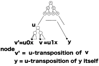
Then, by using a natural isomorphism between the two sub-trees, we can naturally define the concept of u -transposition of a leaf (Fig. 4).
Fig. 4. Transposition of leaves.
A node in the left sub-tree corresponds to another node in the right sub-tree in such a way that the leftmost leaf in the left sub-tree corresponds to the leftmost leaf in the right sub-tree. If a leaf y is not a descendant of u, we define its
u-transposition as to bey itself.
In the same way, we can define the u-transposition of a truth assignment (Fig. 5), and the u-transposition of an algorithm.
[image:3.595.113.224.240.390.2]Formal definitions are as follows.
Fig. 5. Transposition of truth assignments
Definition 4. Suppose that uis an internal node-code. 1) Suppose that v and v′ are node-codes of the same
length. We say “v′ is the u-transposition of v” (in symbol,v′= tpu(v)) if one of the followings holds.
a) There exist i ∈ {0,1} and a string w such that
v=uiw (concatenation) andv′ =u(1−i)w. b) uis not a prefix ofv and it holds thatv=v′. 2) Suppose thatω,ω′ are assignment-codes. We say “ω′
is the u-transposition of ω” (in symbol,ω′= tpu(ω)) if the following holds for each leaf-code v.
ω′(v) =ω(tpu(v))
3) Suppose thatADandA′Dare deterministic algorithms.
We say “A′Dis theu-transposition ofAD” (in symbol,
A′D = tpu(AD)) if the following holds: “For each
assignment-code ω, the query-history of ⟨A′D, ω⟩ is given by applying component-wisetpuoperation to the query-history of ⟨AD,tpu(ω)⟩.” To be more precise,
denote the query-history of ⟨AD,tpu(ω)⟩ and that
of ⟨A′D, ω⟩ by⟨x(1),· · · , x(m)⟩ and⟨y(1),· · · , y(m)⟩,
respectively. Then, the following holds.
∀j≤m y(j)= tpu(x(j))
And, the answer history of ⟨AD,tpu(ω)⟩is the same
as that of⟨A′D, ω⟩.
Example 1. We consider the case where h = 2. Then the followings hold.tpλ(abcd) =cdab, tp0(abcd) =bacd and tp1(abcd) = abdc, where we denote a truth assignment ω
by a stringω(00)ω(01)ω(10)ω(11).
Definition 5. 1) Ais closed (under transposition)if for each AD ∈ A and for each internal node-code u, we
havetpu(AD)∈ A.
2) Ωisclosed (under transposition)if for eachω∈Ωand for each internal node-code u, we have tpu(ω)∈Ω. 3) Ω is connected (with respect to transposition) if for
every distinct members ω, ω′ ∈ Ω, there exists a finite sequence⟨ωi⟩i=1,···,N inΩand a finite sequence
⟨u(i)⟩i=1,···,N−1of strings such thatω1=ω, ωN =ω′
and for each i < N,ωi+1 is theu(i)-transposition of ωi.
IAENG International Journal of Applied Mathematics, 42:2, IJAM_42_2_07
[image:3.595.70.259.490.617.2]ConventionThroughout the rest of the section,Adenotes a non-empty closed subset of AD.
Definition 6. Suppose thatp1,· · ·, pn are non-negative real
numbers such that their sum makes 1. And, suppose that Ω1,· · · ,Ωn are mutually disjoint non-empty families of
assignment-codes. In addition, suppose that d1,· · · , dn are
distributions such that each dj is a distribution onΩj.
1) p1d1 + · · · + pndn denotes the distribution d on
Ω1 ∪ · · · ∪ Ωndefined as follows. For each j (1 ≤
j ≤n) and each truth assignment ω ∈ Ωj, we have
prob[disω ] =pj×prob[ dj isω ].
2) Given a distribution d, we say “d is a distribution on
p1Ω1+· · ·+pnΩn” if there exist distributionsd′j on
Ωj (1≤j≤n) such that d=p1d′1+· · ·+pnd′n.
The following is a variant of the no-free-lunch theorem. Lemma 1. Suppose thatp1,· · ·, pn andΩ1,· · ·,Ωn satisfy
the requirements in Definition 6, and that each Ωj is
con-nected. Then, there exits a real numbercsuch that for every distribution donp1Ω1+· · ·+pnΩn, the following holds.
∑
AD∈A
C(AD, d) =c (1)
Proof: We begin with the case of n = 1. For every assignment-code ω and for every internal node-code u, the mapping ofAD∈ Atotpu(AD)is a permutation ofA. And,
we haveC(tpu(AD), ω) =C(AD,tpu(ω)). Hence, the sum
of C(AD, ω)over all AD∈ Ais the following.
∑
AD∈A
C(tpu(AD), ω) =
∑
AD∈A
C(AD,tpu(ω)) (2)
In the left-hand side, u is fixed, and AD runs over
all elements of A. Thus, tpu(AD) runs over all elements
of A, too. Hence, it holds that ∑A
D∈AC(AD, ω) =
∑
AD∈AC(AD,tpu(ω)). Therefore, since Ω1 is connected, there exists a real number c such that for every ω ∈ Ω,
∑
AD∈AC(AD, ω) =c. Hence, the left-hand side of (1) is equal to the following.
∑
AD∈A
∑
ω∈Ω
prob[d=ω]C(AD, ω)
=∑
ω∈Ω (
prob[d=ω] ∑
AD∈A
C(AD, ω)
)
=c (3)
Thus, the case ofn= 1 is proved.
The general case is as follows. There exist probability distributions di on Ωi (1 ≤ i ≤ n) such that d =p1d1+ · · ·+pndn. By the above proof, there exist positive constants
c1,· · ·, cn such that for each i, (1) holds for di andci in
place ofdandc. Letc=p1c1+· · ·+pncn. Then (1) holds.
Lemma 2. Suppose thatp1,· · ·, pn andΩ1,· · ·,Ωn satisfy
the requirements in Definition 6. And, suppose that eachΩj
is closed.
1) Letdunif.(p1Ω1+· · ·+pnΩn)denote the distribution
p1d1 +· · · + pndn, where each dj is the uniform
distribution on Ωj. Then, there exits a real numberc
such that for every deterministic algorithmAD∈ AD,
it holds thatC(AD, dunif.(p1Ω1+· · ·+pnΩn)) =c.
2) Suppose that each Ωj is not only closed but also
connected and that d is a distribution on p1Ω1 + · · ·+pnΩn. Then, the following (a), (b) and (c) are
equivalent, whereBj are any deterministic algorithms
(not necessarily a member ofA), anddunif.(Ωj)is the
uniform distribution on Ωj.
a) The following holds, whered′runs over distribu-tions onp1Ω1+· · ·+pnΩn.
min
AD∈A
C(AD, d) = max d′ AminD∈A
C(AD, d′) (4)
b) There exits a real number c such that for every AD∈ A, it holds that C(AD, d) =c.
c) min
AD∈A
C(AD, d) = n
∑
j=1
pjC(Bj, dunif.(Ωj)) (5)
Proof: 1. In the same way as the proof of Lemma 1, the case of n ≥2 is reduced to the case of n = 1. Thus, in the following, we prove the case of n= 1 by induction onh. The case ofh= 1is immediate. At the the induction step, letT0(T1, respectively) be the left (right) sub-tree just
under the root. SinceΩ1is closed, the assertion is equivalent
to its weaker form: “The costs are the same for all algorithms which probeT0beforeT1.” We call such algorithms “left-first algorithms” in this proof.
Now,Ω1is partitioned into sets such that each component
Ω′ is of the following form. There exist strings α0 andα1
(depending onΩ′) such thatαi is an assignment-code forTi
for eachi, and the componentΩ′is the direct product of the closure ofα0and that ofα1. Here, the closure ofαi denotes
the following set.
{tpu(αi) : uis an internal node-code} (6)
By the induction hypothesis, the cost of a left-first al-gorithm depends only on Ω′, and does not depend on an algorithm. Hence, the same holds with respect toΩ1.
2. By the assertion 1 of the current lemma and Lemma 1, each of the assertions (a) and (b) is equivalent to (7).
min
AD∈A
C(AD, d) =
1
|A| ∑
AD∈A
C(AD, d) (7)
Therefore, by the assertion 1, (a) is equivalent to the following.
min
AD∈A
C(AD, d) = min AD∈A
C(AD, dunif.(p1Ω1+· · ·+pnΩn))
(8) And, the right-hand side of (8) equals to the right-hand side of (5). Hence, (a) is equivalent to (c).
Lemma 3. Assume thatT is an AND-OR tree. Suppose that dis an eigen-distribution with respect toA(see Definition 3). Thendis a distribution on the 1-set.
Proof:For each positive integerhand each i∈ {0,1}, we let c∧i,h (c∨i,h, respectively) denote C(AD, dunif.(i-set))
for the perfect binary AND-OR tree (OR-AND tree, re-spectively) of height h. Here, AD is an element of A. By
Lemma 2,c∧i,h(c∨i,h) is well-defined regardless of the choice ofAD.
IAENG International Journal of Applied Mathematics, 42:2, IJAM_42_2_07
Claim 1. Suppose thatΩ is closed. If a given tree is an AND-OR tree andΩis not the 1-set (a given tree is an OR-AND tree and Ωis not the 0-set, respectively), then for any deterministic algorithm AD, C(AD, dunif.(Ω)) is less than
c∧1,h(c∨0,h, respectively).
Proof of Claim 1: By induction onh, the following weak form of Claim 1 is shown.
(∗): “Suppose that Ω′ is a non-empty family of truth assignments such that Ω′ is closed. Let i∈ {0,1} be such that for all elements of Ω′, the root has the value i. In addition, suppose thatΩ′ is not thei-set. If a given tree is an AND-OR tree (an OR-AND tree, respectively), then for any deterministic algorithm AD, C(AD, dunif.(Ω′)) is less than
c∧i,h(c∨i,h, respectively).”
And, by induction onh, the followings are shown.
c0∧,h=c∨1,h< c1∧,h=c∨0,h≤ 4
3c ∧,h
0 (9)
Consider the case where the tree in Claim 1 is an AND-OR tree. LetADbe a deterministic alogorithm. In the case where
the root has the value 1 in dunif.(Ω) with probability one,
apply the above mentioned statement (∗) withi= 1. Then we get thatC(AD, dunif.(Ω))< c∧1,h. Otherwise, since we have c∧0,h< c∧1,h by (9), we get thatC(AD, dunif.(Ω))< c∧
,h
1 .
The case where the tree in Claim 1 is an OR-AND tree is shown in the same way. Hence, the claim holds. Q.E.D.(Claim 1)
Now, suppose that T is an AND-OR tree. Suppose that
d is an eigen-distribution with respect toA. Let ⟨Ωj :j =
1,· · · , n⟩ be a partition of the set of all truth assignments to connected closed sets. Without loss of generality, Ω1 is
the 1-set. For each j, let pj be the probability ofd being a
member of Ωj. By Lemma 2, (5) holds. Hence, by Claim
1, there are positive real numbers c2,· · · , cn such that the
following holds.
∀j ≥2 cj< c∧ ,h
1 (10)
min
AD∈A
C(AD, d) =p1c∧1,h+
n
∑
j=2
pjcj (11)
Since dis eigen with respect to A,d achieves the maxi-mum value of (11). Hence, it holds that p1= 1 andpj= 0
for allj≥2. Thus,dis a distribution on the 1-set. Theorem 4. Assume that a given tree T is Tk
2 for some positive integer k. Suppose that a family A of algorithms is closed under transposition and that d is a probability distribution on the assignment-codes. Then, the followings are equivalent (see Definition 3).
(LT1A)dis an eigen-distribution with respect toA. (LT2A)dis an E1-distribution with respect to A.
Proof: By Lemma 3, (LT1A) is equivalent to “d is an eigen-distribution with respect to⟨A,(1-set)⟩”. By Lemma 2, this is equivalent to (LT2A).
IV. ACASE WHERE THE UNIQUENESS FAILS A direct corollary to Lemma 2 is the following.
Corollary 5. Assume that a given tree T is Tk
2 for some positive integerk. Then, (LT3) implies (LT2A):
(LT3)dis the uniform distribution on the 1-set. (LT2A)dis anE1-distribution with respect toA.
We show that the uniqueness of the eigen-distribution fails in the directional case. This is shown by proving that (LT2A) does not imply (LT3) with respect toA=Akdir (see below). Convention Akdir denotes Adir (see Definition 2) in the
case whereh= 2k andT =Tk
2.
TABLE I
C(AD, ω)FORk= 1(ω∈THE1-SET).
A1 A2 A3 A4
1234 4312 3421 2143
ω1 1010 2 3 3 4
ω2 1001 3 2 4 3
ω3 0110 3 4 2 3
ω4 0101 4 3 3 2
A5 A6 A7 A8
3412 1243 2134 4321
ω1 1010 2 3 3 4
ω2 1001 3 2 4 3
ω3 0110 3 4 2 3
ω4 0101 4 3 3 2
For the time being, we investigate the case wherek= 1. Table I shows the values of C(AD, ω) in the case where
ω is an element of the 1-set. In the table, each ωi is the
name of an assignment. We denote an assignment-code ω
by a string ω(00)ω(01)ω(10)ω(11). And, each Aj is the
name of an element of A1
dir. Recall Definition 2. Each Aj
is determined by a permutationxyzwof{0,1}2 that shows
priority of scanning leaves. In the table, a string such as 1234 denotes a permutation of the above property, where we denote leaf-codes 00, 01, 10 and 11 by numerals 1, 2, 3 and 4, respectively. Since we consider alpha-beta pruning algorithms, only the eight permutations are considered. Theorem 6. [9]
1) There are uncountably many E1-distributions with respect to A1dir. Hence, (LT2A) does not imply (LT3) with respect to A=A1
dir.
2) There are uncountably many eigen-distributions with respect to A1
dir.
Proof:1. Suppose that0≤ε≤1/2. By dε, we denote
the distribution don the 1-set such that the probabilities of
d being ω1, ω2, ω3 and ω4 are ε,1/2−ε,1/2−ε and ε,
respectively. Let j ∈ {1,2,· · ·,8}. Note that ε(2 + 4) + (1/2−ε)(3+3) =ε(3+3)+(1/2−ε)(2+4) = 3. Therefore, by Table I, it holds thatC(Aj, dε) = 3. Hence, for everyε
such that0≤ε≤1/2,dεis a distribution on the 1-set, and
the value C(Aj, dε) does not depend on j. And, dε is not
the uniform distribution on the 1-set unlessε= 1/4. The assertion 2 of the theorem is immediate from the assertion 1 and Theorem 4.
On the other hand,E0-distribution with respect toA1 diris
unique. Sketch of the proof is as follows. Table II shows the values of C(AD, ω) in the case where ω is an element of
the 0-set. Now, under the assumption that a distributiondon the 0-set has the same cost for all Aj (1 ≤j ≤8), set up
equations on probabilities ofdbeing equal toωi(5≤i≤8).
IAENG International Journal of Applied Mathematics, 42:2, IJAM_42_2_07
TABLE II
C(AD, ω)FORk= 1(ω∈THE0-SET).
A1 A2 A3 A4
1234 4312 3421 2143
ω5 1000 3 2 2 4
ω6 0100 4 2 2 3
ω7 0010 2 4 3 2
ω8 0001 2 3 4 2
A5 A6 A7 A8
3412 1243 2134 4321
ω5 1000 2 3 4 2
ω6 0100 2 4 3 2
ω7 0010 3 2 2 4
ω8 0001 4 2 2 3
Observe that the upper half of Table II is a matrix of non-zero determinant. And, the lower half of the table is such a matrix, too. Thus, it is easy to see that the equations have a unique solution ofprob[d=ωi] = 1/4 (5≤i≤8), in other
words, dis the uniform distribution on the 0-set.
We close this section with a remark that for each positive integerk, the statements of Theorem 6 hold forAk
dirin place
of A1
dir. In addition, in the case ofk≥2, the uniqueness of E0-distribution fails, too.
Theorem 7. [9]
1) There are uncountably many E1-distributions with respect toAk
dir. Hence, (LT2A) does not imply (LT3) with respect toA=Ak
dir.
2) Ifk≥2, there are uncountably manyE0-distributions with respect toAk
dir.
3) There are uncountably many eigen-distributions with respect toAkdir.
Proof: Suppose that his a positive integer, i is either 0 or 1 and d0 (d1, respectively) is E0-distribution (E1
-distribution) for an AND-OR tree of heighth. Then, we can construct an Ei-distribution for an OR-AND tree of height
h+1in the following way. In the case ofi= 0, we assignd0
to both of the two sub-trees just under the root. Otherwise, letdi,j(i, j∈ {0,1}) denote the truth assignment that assign
dito the left sub-tree and assigndj to the right sub-tree. We
assign(1/2)d0,1+ (1/2)d1,0 to the tree (see Definition 6). A
similar construction is done for the case where the roles of an AND-OR tree and that of an OR-AND tree are interchanged. Hence, by Theorem 6 and an induction on the height of a tree, we get the current theorem.
V. ACASE WHERE THE UNIQUENESS HOLDS In this section, we give an alternative proof for the characterization of the eigen-distribution (in the usual case) as the uniform distribution on the 1-set [4]. To be more precise, we show that (LT2A) implies (LT3) with respect to the non-directional algorithms (see Corollary 5).
An example of an element ofA1D− A1diris the following algorithm. It begins with scanning the leaf of code 00. If a beta-cut does not happen there, the query-history is
⟨00,01,10,11⟩. Otherwise, the query-history is⟨00,11,10⟩, where the leaf-code 01 is skipped due to the beta-cut. By taking transpositions of this algorithm, we know that
A1
D− A
1
dir consists of 8 algorithms.
Theorem 8. [5] Suppose thath≥2, wherehis the height ofT. Then, (LT2A) implies (LT3) with respect toA=AD−
Adir.
Proof:For each i∈ {0,1} and a positive integer g, let (i-set)g denote thei-set in the case of h=g. By induction onh≥2, we shall show the following requirementRh.
Rh: “Suppose thati∈ {0,1} and that a distributiondon
(i-set)his anEi-distribution with respect toA=A
D−Adir.
Then,dis the uniform distribution on (i-set)h.”
The base caseR2is shown by solving equations; it is in the
same way as our proof of the uniqueness ofE0-distribution
with respect toA1 dir.
Suppose thatRn holds. In the rest of the proof, let h=
n+ 1, i ∈ {0,1} and assume that d is a distribution on (i-set)n+1 and that d is an Ei-distribution with respect to
AD− Adir. We investigate the case where the root is an
AND-gate andi= 1. The other cases are shown in the same way.
Let T0 (T1, respectively) be the left (right) sub-tree just
under the root. For each assignmentαonT0 (such thatα∈
(1-set)nand the denominator of (12) is positive), consider the distributiondα onT1 as follows. For each assignmentβ on T1, we letprob[dαis β ]as to be the following conditional
probability, whereαβdenotes the concatenation ofαandβ. prob[dis αβ | ∃x disαx ] (12) By the induction hypothesis Rn, for allα such thatα∈
(1-set)n and the denominator of (12) is positive, d α is the
uniform distribution on (1-set)n. The same holds for the case
where the roles ofT0 andT1 are exchanged.
Now, by the induction hypothesisRn, it is not hard to see
that the requirementRn+1 is satisfied.
VI. CONCLUSIVE REMARKS
By extending the work of Tarsi [11], it is shown by Saks and Wigderson that the randomized complexity of an AND-OR tree is the same as that for directional algorithms; for more pricise, see [8, Theorem 5.2]. In the case of T2k, by using our results in § III, the above result is extended as follows.
Proposition 9. Suppose thatkis a positive integer andT is Tk
2. And, suppose that Ais a non-empty subset of AD and
Ais closed under transposition. Then, the following holds, wheredruns over all distributions.
max
d ADmin∈AD
C(AD, d) = max
d Amin∈AC(AD, d) (13)
Proof: Letdunif. be the uniform distribution on the
1-set. By Lemma 2 and Lemma 3, the both sides of (13) are equal to the following.
min
AD∈AkD
C(AD, dunif.) = min AD∈A
C(AD, dunif.)
Hence, the AD (the class of all deterministic algorithms
for the tree) andAdir(that of all directional algorithms) have
the same distributional complexity.
IAENG International Journal of Applied Mathematics, 42:2, IJAM_42_2_07
In contrast, they do not agree on the question of “Which distribution achieves the equilibrium?” A variant of the no-free-lunch theorem implies the equivalence of “eigen” and “E1”, but it does not imply the uniqueness of the
eigen-distribution. The set of all un-directional algorithms plays an important role to show the uniqueness.
ACKNOWLEDGMENT
The authors would like to thank M. Kumabe, C.-G. Liu, Y. Niida, K. Tanaka and T. Yamazaki for helpful discussions.
REFERENCES
[1] Arora, S. and Barak, B.: Comput. Complex., Cambridge university press, New York, 2009.
[2] Ho, Y.C. and Pepyne, D.L.: Simple explanation of the no-free-lunch theorem and its implications.J. Optimiz. Theory App.,115pp.549– 570 (2002).
[3] Knuth, D.E. and Moore, R.W.: An analysis of alpha-beta pruning.
Artif. Intell.,6pp. 293–326 (1975).
[4] Liu, C.-G. and Tanaka, K.: Eigen-distribution on random assignments for game trees.Inform. Process. Lett.,104pp.73–77 (2007). [5] Nakamura, R.: Randomized complexity of AND-OR game trees.
Master thesis, Department of Mathematics and Information Sciences, Tokyo Metropolitan University, Tokyo (2011).
[6] Pearl, J.: Asymptotic properties of minimax trees and game-searching procedures.Artif. Intell.,14pp.113–138 (1980).
[7] Pearl, J.: The solution for the branching factor of the alpha-beta pruning algorithm and its optimality.Commun. ACM,25pp.559–564 (1982).
[8] Saks, M. and Wigderson, A.: Probabilistic Boolean decision threes and the complexity of evaluating game trees. In: Proc. 27th Annual IEEE Symposium on Foundations of Computer Science (FOCS), pp.29–38 (1986).
[9] Suzuki, T.: Failure of the uniqueness of eigen-distribution on random assignments for game trees.S¯urikaisekikenky¯usho-Kokyuroku,1729 pp.111–116, Research Institute for Mathematical Sciences, Kyoto University (2011).
[10] Suzuki, T. and Nakamura, R.: Probability distributions achieving the equilibrium of an AND-OR tree under directional algorithms. Lecture Notes in Engineering and Computer Science: Proceedings of The International MultiConference of Engineers and Computer Scientists 2012, IMECS 2012, 14-16 March, 2012, Hong Kong, pp.194-199. [11] Tarsi, M.: Optimal search on some game trees.J. ACM,30pp. 389–
396 (1983).
[12] Wolpert, D.H. and MacReady, W.G.: No-free-lunch theorems for search,Technical report SFI-TR-95-02-010, Santa Fe Institute, Santa Fe, New Mexico (1995).
[13] Yao, A.C.-C.: Probabilistic computations: towards a unified measure of complexity, in:Proc. 18th annual IEEE symposium on foundations of computer science (FOCS), pp.222–227 (1977).
![TABLE II (ω 0-). T. Then, (LT2 [5] Suppose thatofTheorem 8.A) implies (LT3) with respect to, where is the height FOR k = 1 ∈ THESET h ≥ 2 h A = AD −](https://thumb-us.123doks.com/thumbv2/123dok_us/385988.536113/6.595.88.251.57.187/table-suppose-thatoftheorem-implies-respect-height-theset-ad.webp)
