An Efficient and Cost Saving Component Scheduling Algorithm Using High Speed Turret Type Machines for a Board Containing Multiple PCBs

doi:10.4236/ica.2011.22010 Published Online May 2011 (http://www.SciRP.org/journal/ica)

An Efficient and Cost-Saving Component Scheduling

Algorithm Using High Speed Turret Type Machines for a

Board Containing Multiple PCBs

Wei-Shung Chang, Chiuh-Cheng Chyu

Department of Industrial Engineering and Management, Yuan-Ze University, Chinese Taipei E-mail: s948905@mail.yzu.edu.tw, [email protected]

Received January 6, 2011; revised March 28, 2011; accepted April 2, 2011

Abstract

This paper considers a material constrained component scheduling problem during the high speed surface mount manufacturing stage in printed circuit board (PCB) assembly, where each piece of board contains an even number of identical PCBs. To accomplish the production, material requirements must be predetermined and incorporated as restraints into the scheduling problem, which has the objective of minimizing production completion time (makespan). A solution procedure is developed based on the following strategies: 1) Each machine is responsible for the same PCBs of each piece, 2) Components of the same types may use one or more feeder locations, 3) Component types are clustered based on their suitable placement speeds, 4) A heu-ristic using a bottom-up approach is applied to determine the component placement sequence and the feeder location assignment for all machines. Velocity estimate functions of the turret, XY table, and feeder carriage were derived based on empirical data. An experiment using Fuji CP732E machines was conducted on two real life instances. Experimental results indicate that our method performs 32.96% and 10.60% better than the Fuji-CP software for the two instances, in terms of the makespan per piece of board.

Keywords:Printed Circuit Boards Assembly, Surface Mount Technology, Heuristics, Component Placement Sequence, Feeder Location Assignment

1. Introduction

In printed circuit board (PCB) assembly, surface mount technology (SMT) is extensively used to populate boards with electronic components. The tools implementing SMT are generally called surface mount device (SMD) placement machines. Based on specifications and opera-tional methods, the SMD are classified into five categories [1]: dual-delivery, multi-station, turret-type, multi-head and sequential pick-and-place. High-speed chip place-ment machines belong to the turret-type.

In many SMT assembly lines, the SMD processing is most likely the bottleneck of production, especially when the number of components on a PCB is large, or when a piece of board contains several identical PCBs. The most prevalent analytical approach is to hierarchically de-compose the problem into a number of more easily manageable subproblems, and solve each subproblem one at a time. The solution to the global problem can then be obtained by integrating the subproblems’

solu-tions. Several researchers [1] presented similar hierar-chical classification schemes for the task. Their classifi-cation is based on the number of machines (one or many) and the number of board types (one or many) present in the problem. This paper studies the component place-ment problem using turret style surface mount placeplace-ment machines for PCBs; the problem becomes increasingly complicated when greater operational efficiency is re-quired. This problem usually consists of the feeder loca-tion assignment (FLA), component placement sequence (CPS), and component retrieval problem (CRP) [2]. The CRP permits a component type to use more than one feeder slot, and a retrieval plan must be determined for such component types before production.

focused on the feeder arrangement problem. Their com-putational results indicate that a retrieval plan may merely increase inventory cost but not decrease cycle time. The algorithm by Crama [3] and Klomp [5] is based on the strategy of determining FLA first and CPS next. Under this strategy, an estimation procedure was developed to assess and improve the quality of an FLA solution. Ellis et al. [6] solved the same case by deter-mining CPS first and FLA next. Ong et al. [7], Wu and Ji [8], Chyu and Chang [9] applied the genetic algorithm to solve the CPS and FLA problems simultaneously on one machine and one board type case. Kumar and Luo [10] presented a different approach to optimize the operation sequence using a generalized-TSP model on the same problem. Moon [11] proposed 5-in-1 and 3-in-1 working group assembly methods to solve CPS and FLA prob-lems simultaneously. His computational results indicate that the 5-in-1 procedure performs better in the sin-gle-layered board case, while the 3-in-1 procedure is more effective for the multiple-layered board. Knuutila et al. [12], Narayanaswami and Iyengar [13], Salonen et al. [14] and Jeong [15] presented several grouping PCB assembly jobs strategies for PCB setup time reduction.

This research was motivated during a consultation with a PCB manufacturer. One problem often encoun-tered during PCB assembly is that using leftover com-ponents will increase the frequency of discontinuing production process, but disposing them will incur mate-rial waste cost. Thus, there is a conflict between produc-tion efficiency and material cost saving. A two-phase solution procedure is proposed: Phase 1 aims to carefully plan the material requirements for production scheduling, and Phase 2 searches for a near optimal solution accord-ing to Phase 1 results. Phase 2 is a multi-start heuristic based on the bottom-up strategy, i.e., using CPS first and FLA second, to solve component scheduling problems.

This paper uses Fuji CP 732E machines for the study example. All relevant information, including the data for deriving estimation functions and two real life instances, was obtained via assistance from the manufacturer.

The remainder of the paper is organized as follows: Section 2 describes the problem; Section 3 presents the algorithms; Section 4 presents and discusses the experi-mental results of the algorithms; Section 5 concludes the paper.

2. Problem Description

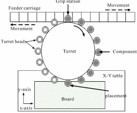
A turret style surface mount placement machine, Fuji CP 732E as shown in Figure 1, consists of three elements: a X-Y table, a feeder rack, and a turret. The X-Y table can move simultaneously in horizontal direction as well as in vertical direction with a PCB on it. The feeder rack

con-sists of the so-called slots. A feeder stores components of a single type and is attached to a slot to the rack. The turret transports components from the rack to the board. Throughout this paper, the term feeder carriage and feeder rack are used interchangeably.

Figure 1 illustrates the operation manner of the ma-chine. The turret moves clockwise and has 16 placing heads positioned evenly apart in a circular manner. The head of the turret at the position of grip station retrieves a component from a feeder attached in a pre-specified slot on the feeder rack, while the head of the turret at the placement station simultaneously mounts a component at a pre-specified location on the PCB. It should be noted that the component gripping sequence and the compo-nent placement sequence are the same but the former is eight ahead of the latter. The first eight turret rotations only pick up components, and the movement time for each pickup is the greater time value between the rota-tion of turret starota-tion and the corresponding shift of the feeder carriage. On the other hand, the last 8 movements are only for placing components on the PCB and the movement time is the maximum value of X-Y table moving time and turret rotation time. As for the turret rotations in between, the movement time is the maximum time value of all three mechanism movements.

Because the PCB table can move both in the vertical and horizontal axes simultaneously, the distance measure between two components on the board is a Chebychev metric, i.e., max





, i j y y

The velocity of the turret has multiple settings. In general, the velocity setup is between 30% and 100%. Components of larger size or heavier weight require a slower velocity to achieve placement accuracy. In practice,

one commonly used feeder arrangement policy is to as-sign full velocity to the smaller sized component typeswith a large population. For any velocity setting, the average velocity increases as the distance traveled increases, although the relationship does not appear to be linear. Larger or heavier components are more difficult to be held accurately during turret rotations; thus, a slower rotation rate is required for such components. The time for any single turret rotation is determined by the component transported with the slowest rotation rate. The machine will perform a grip and a placement opera-tion at the same time after the three mechanisms com-plete their individual movements.

In many cases, the production rate is higher when a component type is allowed to use at least two feeder slots (feeder duplication). In this situation, a decision so-called the component retrieval problem occurs as to which feeder slot should be used to handle the placement job of each component that uses multiple feeder slots. Some researchers address different a point of view for feeder duplication based on inventory cost aspect, even though the duplication can reduce the cycle time. Rosenblatt and Lee [16] discussed the trade-off between inventory cost and throughput rates of the two feeder slot alternatives. Crama et al. [3] suggested that two feeder slots be used while necessary. The experimental results in Klomp et al. [5] indicate that there is no advantage in cycle time re-duction with the use of feeder duplication.

The global problem with one or more machines can be described as follows: Firstly, decide which component types should use feeder duplications; secondly, deter-mine the feeder location assignment (FLA) and CPS for each machine. The CPS problem of a machine is a trav-eling salesman problem (TSP) given an FLA to the ma-chine. The global problem is NP-hard since its sub-problem CPS in each machine is NP-hard. The ob-jective of the problem is to find an FLA and its corre-sponding CPS for each machine such that the production time of each PCB is minimized.

The following are notations and decision variables when a set of components has been assigned to a single machine. This set can be a subset of components in a PCB or all components in one PCB.

K: Total number of component types used in the set. k: Component type index. k = 1,, K.

N: Total number of components in the set. n: CPS index. n = 1,, N.

n

i tp

: The nth component in the CPS. ( )_in

( )

: Component type index for component _in.

f k : Feeder slot number for component type k. ( )

u s : Time for feeder carriage to move s slots leftward or rightward; u(0)0.

1 )

n _in

( ,

v i : Movement time of X-Y table from

com-ponents in to n1

i  . [n

trt i ]: Turret rotation time for component in.

 







 













 







 

























Max , Max

,

Max ,

Max( , ,

n n q

q n n

N

n n

n

q n n

n q n

N

q n n

n q N n N

f tp i f tp i trt i

u f tp i f tp i

trt i v i i

trt i v i i

                 8    Max Max

u _{ }

         _{ }







In the case where two or more identical PCBs are as-signed to one machine, the same FLA will be used. The machine will process these PCBs one by one using this FLA alternatively forwards and backwards. The turret speed changes from fast to slow when processing a PCB with a forward FLA, and from slow to fast when proc-essing one with a backward FLA. In general, there is little difference in processing time between a PCB with forward FLA and a PCB with a backward FLA, but the time that the machine needs to move to the start position of the next PCB needs to be counted.

3. Estimating Velocity Functions

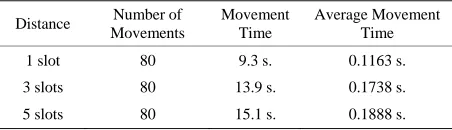
In order to evaluate the performance of our proposed algorithms, experiments were conducted to develop the velocity estimate functions of the turret, XY table, and feeder carriage for the Fuji CP 732E machine. In the ex-periment for estimating the velocity function of the feeder carriage, three trials are devised for measuring the movement speed on each of the three distances, the 1, 3, and 5 slot [17]. Each trial was performed 80 times back and forth. The average value of the three trials for each distance is used as the estimate of the velocity for that distance. Table 1 displays the results of the experiment. The average times for the three distances are approxi-mately 0.1163, 0.1738, and 0.1888 seconds, respectively. Figure 2 shows the plot of the average movement times. It should be noted that the velocity of the feeder carriage is the slowest among the three mechanisms. Usually, the production planner will schedule component placements that require the feeder carriage to shift no more than five slots in one movement.

Table 1. Experimental results of the feeder carriage move-ment time (in seconds).

Distance Number of Movements

Movement Time

Figure 2. Feeder carriage average movement time data plot.

Based on the data in Table 1, a plot for the feeder car-riage average velocity ranging from one to five slots is shown in Figure 2. An estimation formula for the veloc-ity is given as follows.

 

x x

V x

x x

 



  _{ }





 (2)

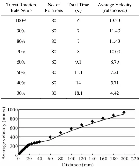
To determine the average velocity of the turret rotation including pick and place, an experiment was conducted and the results are shown in Table 2. This experiment includes eight different turret rotation rate setups, from the slowest speed of 30% to the full speed of 100%. For each rate setup experiment, three trials of 80 consecutive rotations are performed and the average of the three movement times is taken as the estimate. The experi-mental results are shown in Table 2 and the velocity plot is presented in Figure 3.

4. Problem Solving Procedure

This paper focuses on the component scheduling prob-lem that arises in the high speed surface mount manu-facturing stage of PCB assembly, where each board piece contains an even number of identical PCBs and the pro-duction stage may involve more than one machine. It is thus reasonable to assume that the number of machines used in the production line should be a number divisible by the PCBs in the board. For example, if a board piece contains two identical PCBs, then the number of ma-chines can be one or two.

The proposed solution procedure aims to minimize the production completion time (makespan), where the ma-terial availability constraints are imposed for cost-saving purposes. This solution procedure adopts the following policies: 1) Have each machine be responsible for the same number of PCBs of each piece, 2) Find the maxi-mum number of feeder slots that a component type can use for each machine and, allowing feeder duplications, calculate all alternatives for the number of feeder slots used for a machine, 3) Cluster the component types based on their suitable placement speeds and then proc-esses the groups one by one with speeds from high to low, 4) Apply a multi-start local heuristic using nearest

Table 2. Experimental results on the velocity of the turret rotation involving pick and placement.

Turret Rotation Rate Setup

No. of Rotations

Total Time (s.)

Average Velocity (rotations/s.) 100% 80 6 13.33

90% 80 7 11.43 80% 80 7 11.43 70% 80 8 10.00 60% 80 9.1 8.79 50% 80 11.1 7.21 40% 80 14 5.71 30% 80 18.1 4.42

Figure 3. XY-Table velocity.

neighbor search with 2-opt or 3-opt to determine the component placement sequence and the feeder location assignment for all machines.

When a machine is assigned to manufacture at least two PCBs in a piece of a board, a promising solution would be to apply the CPS in forward order on one PCB, in reverse order on the next PCB, and so forth until all of the PCBs for which this machine is responsible have been completed. This strategy has been proven effective and efficient in simulation and can be applied in practice.

4.1. Feeder Duplication

The use of feeder duplication is subject to two conditions: 1) material availability and 2) production efficiency. A feeder duplication of a component type should be used if it can increase the production rate and enough quantity is provided. In general, if components of a type are distrib-uted in a scattered manner, then feeder duplication may reduce the tardiness resulting from the XY table due to long distance travels. The following discusses some ma-terial restrictions imposed on the feeder duplication of a component type:

10 components of a certain type, and a reel of such a component type contains 3000 units. Suppose the order demands 5000 units of the PCB type. Thus, 16.67 reels of this component type will be required in this order. Since the reel is not divisible, a minimum of 17 reels will meet the requirement. Adding one reel to make 18 reels in total will allow feeder duplication with 2 or 3 slots, but this would imply that 1.33 reels of components are wasted. In reality, only 17 reels will be used if such components are expensive. In Table 3, the third compo-nent type will not be appropriate for feeder duplication because the number of reels required is 7. Having a large number of feeder duplications for a component type in general will cause a negative impact on the production efficiency.

Another restriction comes from the number of slots available in the machine. The Fuji CP 732E has 60 feeder locations. In our experiment, sample 1 PCB re-quires 56 component types, so the use of feeder duplica-tion is highly limited in this case.

The number of components required by this type must be divisible by the number of feeder locations used. A choice of clusters with unequal number of components will cause material waste. In Table 3, the second type requires 5 components. A 2-cluster with (3, 2) or (1, 4) will therefore likely result in material waste, and fur-thermore, such a choice will not be appropriate when the availability of such material is limited.

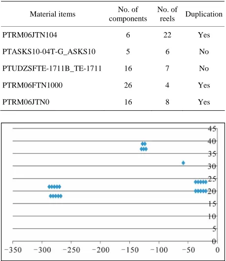
In general, a suitable choice for the number of feeder duplications will reduce the production cycle time. Fig-ure 4 displays the distribution of the fourth component type shown in Table 3. It can be perceived that using one duplication with a 2-cluster (10, 16) or three duplications with 4-cluster (10, 5, 1, 10) for this component type will improve the production efficiency, but five or more will cause a negative effect. The speed of feeder carriage movement is the slowest among the three mechanisms shown in Figure 1. An n-feeder duplication of a compo-nent type would imply that there will be n additional one-slot movements of the feeder carriage. In general, feeder duplication will not improve production efficiency if the n is large. Moreover, with the limitation on the resource availability, we will choose a number of clusters so that each has the same number of components. Based on the above arguments, at most n = 2 feeder duplica-tions will be considered for the problem under study.

A two-step scheme is proposed for deciding all feeder duplications of a PCB.

Step 1: For each component type, we first check if the type violates restrictions (1) and (3) for n = 1 or 2. If not, apply the nearest neighbor method (NNS) to find a Ham-iltonian cycle. The processing time of each arc in this cycle is Max{one stop turret rotation time, XY table

Table 3. Information of some material items.

Material items No. of components

No. of

reels Duplication

PTRM06JTN104 6 22 Yes PTASKS10-04T-G_ASKS10 5 6 No

PTUDZSFTE-1711B_TE-1711 16 7 No PTRM06FTN1000 26 4 Yes PTRM06JTN0 16 8 Yes

Figure 4. The location distribution of components of type PTRM06FTN1000 in sample 1.

movement time}. The estimated processing time of a component type is defined as the path produced by de-leting the maximum time arc from the corresponding Hamiltonian cycle. Let C denote the set of the candidates for feeder duplication. Repeat the following step until either all feeder locations are filled or no more feeder duplication is possible.

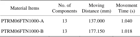
Step 2: Select the component type with the largest es-timated processing time, say, T, in C. Find the best 2-partition (n = 1) or 3-partition (n = 2) of this compo-nent type using the Hamiltonian cycle computed in step 1. All partitioned subsets or clusters contain an equal num-ber of components. If both cases can be chosen, we take n = 1. Let Tidenote the estimated processing time for the ith cluster. For the case of n = 1, if T1 + T2 + one feeder location movement time > T, then duplication is rejected; otherwise, it is accepted. When accepted, update C and each new cluster will be treated as an independent com-ponent type. Go to Step 2. In the case of n = 2, the rejec-tion condirejec-tion is T1 + T2 + T3 + two feeder locations movement time > T.

Table 4. Results of the movement time of each component type in the duplication candidate set.

Material Items No. of Components

Moving Distance (mm)

Processing Time (s) PTRM06FTN1000 26 316.190 2.134a

PTRM06JTN0 16 115.540 1.194 PTRM06JTN104 6 85.960 0.478 PTKC20E1A106MTS 6 56.300 0.429

a: maximum processing time.

Table 5. Results of feeder duplications for the selected component type.

Material Items No. of Components

Moving Distance (mm)

Movement Time (s) PTRM06FTN1000-A 13 137.000 1.040 PTRM06FTN1000-B 13 177.150 1.018

2.134. Thus this component type will be rejected for feeder duplication. Then we continue on to process the component type in the second row of Table 4.

4.2. Clustering Component Types

Component types using similar turret speed settings are clustered into a group. Suppose that there are a total of M groups, with group m using the mth velocity setting of the turret. The speed for the mechanism decreases as m in-creases, which implies that larger and heavier compo-nents will be processed with a slower velocity. The grouping strategy is very time-saving since the turret velocity will be decreasing in a stepwise manner instead of having large variation of up-and-downs in the manu-facturing process.

4.3. Multi-Start Bottom-up Strategy Heuristic

The bottom-up strategy for solving the component scheduling problem is to find a CPS first while at the same time determining the corresponding FLA. Under this strategy, the components of the same type are treated as an individual group. Then the nearest neighbor search (NNS) is applied to each group to find the component placement sequence of that group. In the process, the choice of the next group is determined by the component type that is not processed and has a component located closest to the last component in the last group. Then a local refinement is applied to improve the component placement sequence of each group.

The following describes the problem solving proce-dure, which consists of two phases.

4.3.1. Phase 1: Preprocessing

Apply the two-step feeder duplication procedure de-scribed in Section 4.1 and determine the set of compo-nent types that will use feeder duplications. For each of these component types, identify the components in each subgroup. It should be noted that each subgroup will be regarded as a different type, even though they are of the same component type. Let m be the set of component types using a rotary turret with speed index m = 1,, M. Feeder location has index r = 1, , R.

4.3.2. Phase 2: Multi-Start Bottom-up Solution Procedure

Process the groups of components {1,, M} sequen-tially. Start with 1 and r = 1.

Step 1: Process components in 1.

Step 1.1: Among all components in 1, select a com-ponent c1 that is closest to the origin. Starting with com-ponent c1, compute the CPS for the remaining compo-nents of type tp(c1) with the NNS method. We denote the CPS for tp(c1) as CPS_1. Assign component type tp(c1) to feeder location with index 1. Set r = 2; 1 = 1/tp(c1).

Step 1.2: Seek a component cr in 1, that is closest to the last component of CPS_r-1. Compute the CPS for the remaining components of tp(cr) using the NNS method. Assign component type tp(cr) to feeder location r. 1 = 1/tp(cr). Set r = r + 1.

Step 1.3: If 1 = , set m = 2 and proceed to Step 2; otherwise return to Step 1.2.

Step 2: First, find the component in m that is closest to the last component in the CPS for m-1. Apply the same procedure used in Steps 1.2 and 1.3 for m, and then repeat Step 2 until m = M.

Step 3: For each CPS_r, excluding the first and last components, apply 2-opt for small-size groups (10 components) and 3-opt for medium to large-size groups to make additional refinements. Output the final solution after all the CPS_r have been refined.

5. Experimental Result

Figure 5. A sample piece containing two identical PCBs.

Figure 6. A sample piece containing four identical PCBs.

Table 6. Number of components and types in the sample piece.

PCB board Length (mm)

Width (mm)

Component

Types per PCB Components in Total Sample 1 351.5 93 56 350 (175 per PCB) Sample 2 236 116.3 38 496 (124 per PCB)

processor and 1.0 GB DDR RAM. Experiments are con-ducted with one and two Fuji CP732E placement ma-chines with 60 feeder slots. The estimation functions for the velocities of the feeder carriage, turret, and X-Y table presented in Section 3 will be used for calculating the cycle times of both samples.

An experiment using these two sample pieces is con-ducted in testing the performance of the proposed prob-lem solving procedure described in Section 4.3. For ei-ther PCB, the component types are classified into three categories: 1, 2 and 3, where the components in 1, 2 and 3 are processed at 100%, 80%, and 50% of the full turret rotation rate, respectively. In sample 1, 1 contains 46 types with a total of 151 components, 2 contains 9 types with a total of 23 components, and 3 has only one component; In sample 2, 1 contains 33 types with a total of 112 components, 2 contains 3 types with a total of 11 components, and 3 has only one component.

The experiment contains two cases: one-machine and two-machine. In the one-machine case, the cycle time of a solution is measured by two methods and the deviation is calculated. The two methods are as follows: 1) the cycle time is calculated using the estimation functions

and 2) the solution is implemented on the machine using the commercial software, Fuji-CP. The two-machine case measures the cycle time by the proposed algorithm using estimation functions, and by directly employing the Fuji-CP software. The deviation between the two is then calculated. The results indicate the algorithm out-performs commercial Fuji-CP software in terms of cycle time.

Table 7 presents the computational results of the algo-rithm in the one-machine case for both samples based on the estimation functions. In both samples, feeder dupli-cation is not applied using the algorithm in Section 4.1. Table 8 shows the cycle time deviations between com-puter results and on-line implementation of the solutions in Table 7. The cycle time deviation is defined as the subtracted difference divided by the computer simulation result. From Table 8, we observe that the deviations are very small for both samples, 0.76% for sample 1 and 0.48% for sample 2. This shows that the computer simu-lation results can be used to estimate solution perform-ance for the two real life instperform-ances in the two-machine case.

Both samples in the two-machine case are consecu-tively solved three times by the multi-start algorithm, and the average values are used for the further performance estimation. Table 9 displays the computational results based on the three runs. As we can perceive from this table, the processing times are quite close for the ma-chines, regardless of which sample. Thus, the algorithm will provide workload-balancing solution. In addition, small standard deviations indicate that the algorithm is robust in finding near optimal solutions. Table 10 pro-vides the estimated processing time for implementing each sample onto each machine. The estimation is calcu-lated by adding the deviation.

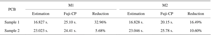
Table 11 presents the estimated improvements when these solutions are implemented online. In the two-ma-chine case, the cycle time of a sample is the maximum value of the two machines’ processing times. Thus for sample 1, the cycle time is max{25.10, 20.15} = 25.10 when Fuji-CP software is used and is max{16.827, 16.828} = 16.828 when the proposed algorithm is used, which results in approximately (25.10 – 16.828)/25.10 = 32.96% improvement. For sample 2, there is an im-provement of about 10.60%. The result indicates that the algorithm yields a better production efficiency for a

Table 7. Computer results in single machine using the esti-mation functions.

PCB Boards Cycle Time CPU Time Sample 1 34.09 s. 1.963 s. Sample 2 45.90 s. 1.872 s.

Table 8. Deviation between the computer results and online implementations in single machine.

Sample 1 Sample 2

Simulation Implementation Deviation Simulation Implementation Deviation 34.09 s. 34.35 s. 0.76% 45.90 s. 46.12 s. 0.48%

Table 9. Computer results of the algorithm with two machines using the estimation formulae (three runs).

PCB Boards in Machine Minimum Cycle Time Average Cycle Time Stand Deviation Average CPU Time Sample 1_M1 16.680 s. 16.700 s. 1.06% 12.336 s. Sample 1_M2 16.681 s. 16.701 s. 1.11% 12.263 s. Sample 2_M1 22.884 s. 22.913 s. 1.50% 15.234 s. Sample 2_M2 22.912 s. 22.936 s. 1.54% 15.425 s.

Table 10. Estimation on the cycle times of both samples taking into account the deviation.

M1 M2 PCB

Simulation Deviation Estimation Simulation Deviation Estimation Sample 1 16.700 s. 0.76% 16.827 s. 16.701 s. 0.76% 16.828 s. Sample 2 22.913 s. 0.48% 23.023 s. 22.936 s. 0.48% 23.046 s.

Table 11. Estimated improvements for the computed solutions being implemented.

M1 M2 PCB

Estimation Fuji-CP Reduction Estimation Fuji-CP Reduction Sample 1 16.827 s. 25.10 s. 32.96% 16.828 s. 20.15 s. 16.49% Sample 2 23.023 s. 24.41 s. 5.68% 23.046 s. 25.78 s. 10.60%

board with anti-symmetrical configuration than a board with side by side configuration. In contrast to the present method, the Fuji-CP software adopts a different strategy to process a piece of board containing several identical PCBs. Instead of processing its assigned PCBs one at a time, each machine processes all of its assigned PCBs at the same time and place components across these PCBs.

6. Conclusions

Surface mount technology (SMT) has been widely used in PCB assembly for years. In many SMT assembly lines, high-speed chip placement machines are likely the bot-tleneck of production. This paper considers a material constrained component scheduling problem arising at the high speed surface mount manufacturing stage in printed circuit board (PCB) assembly, where each piece of board contains an even number of identical PCBs. A solution procedure to minimize the makespan was developed us-ing a strategy which considers the possibility of feeder duplication and clustering the component types accord-

ing to their suitable velocity setup on turret rotation, to-gether with a multi-start local heuristic using nearest neighbor search with 2-opt or 3-opt procedures im-provement. Velocity estimation functions of the turret, XY table, and feeder carriage were also derived based on empirical data. Experiments with one and two Fuji CP732E machines on two samples demonstrated that the proposed solution procedure is more effective when compared to the Fuji-CP software for these particular instances.

7. References

[1] M. Ayob and G. Kendall, “A Survey of Surface Mount Device Placement Machine Optimisation: Machine Clas-sification,” European Journal of Operational Research, Vol. 186, No. 3, 2008, pp. 893-914.

doi:10.1016/j.ejor.2007.03.042

Flexi-ble Manufacturing Systems, Vol. 8, No. 4, 1996, pp. 287-312. doi:10.1007/BF00170016

[3] Y. Crama, O. E. Flippo, J. V. D. Klundert and F. C. R. Spieksma, “The Assembly of Printed Circuit Boards: A Case with Multiple Machines and Multiple Board Types,” European Journal of Operational Research, Vol. 98, No. 3, 1997, pp. 457-472.

doi:10.1016/S0377-2217(96)00228-7

[4] K. Ohno, Z. Jin and S. E. Elmaghraby, “An Optimal As-sembly Mode of Multi-Type Printed Circuit Boards,”

Computers and Industrial Engineering, Vol. 36, No. 2, 1999, pp. 451-471. doi:10.1016/S0360-8352(99)00142-4 [5] C. Klomp, J. V. D Klundert, F. C. R. Spieksma and S.

Voogt, “The Feeder Rack Assignment Problem in PCB Assembly: A Case Study,” International Journal of Pro-duction Research, Vol. 64, No. 1, 2000, pp. 399-407. [6] K. P. Ellis, F. J. Vittes and J. E. Kobza, “Optimizing the

Performance of a Surface Mount Placement Machine,”

IEEE Transactions on Electronics Packaging Manufac-turing, Vol. 24, No. 3, 2001, pp. 160-170.

doi:10.1109/6104.956801

[7] N. S. Ong and W. C. Tan, “Sequence Placement Planning for High-Speed PCB Assembly Machine,” Integrated Manufacturing Systems, Vol. 13, No. 1, 2002, pp. 35-46. doi:10.1108/09576060210411495

[8] H. Wu and P. Ji, “A Genetic Algorithm Approach to Op-timizing Component Placement and Retrieval Sequence for Chip Shooter Machines,” International Journal of Advanced Manufacturing Technology, Vol. 28, No. 5, 2006, pp. 556-560. doi:10.1007/s00170-004-2390-2 [9] C. C. Chyu and W. S. Chang, “A Genetic-Based

Algo-rithm for the Operational Sequence of a High Speed Chip Placement Machine,” International Journal of Advanced Manufacturing Technology, Vol. 36, No. 9-10, 2008, pp. 918-926. doi:10.1007/s00170-006-0918-3

[10] R. Kumar and Z. Luo, “Optimizing the Operation Se-quence of a Chip Placement Machine Using TSP Model,”

IEEE Transactions on Electronics Packaging Manufac-turing, Vol. 26, No. 1, 2003, pp. 14-21.

doi:10.1109/TEPM.2003.813002

[11] G. Moon, “Efficient Operation Methods for a Component Placement Machine Using the Patterns on Printed Circuit Boards,” International Journal of Production Research, Vol. 48, No. 10, 2010, pp. 3015-3028.

doi:10.1080/00207540802553608

[12] T. Knuutila, M. Hirvikorpi, M. Johnsson and O. Neva- lainen, “Grouping PCB Assembly Jobs with Feeders of Several Types,” International Journal of Flexible Manu-facturing Systems, Vol. 16, No. 2, 2004, pp. 151-167. doi:10.1023/B:FLEX.0000044838.12637.0e

[13] R. Narayanaswami and V. Iyengar, “Setup Reduction in Printed Circuit Board Assembly by Efficient Sequenc-ing,” International Journal of Advanced Manufacturing Technology, Vol. 26, 2005, pp. 276-284.

doi:10.1007/s00170-003-1634-x

[14] K. Salonen, J. Smed, M. Johnsson and O. Nevalainen, “Grouping and Sequencing PCB Assembly Jobs with Minimum Feeder Setups,” Robotics and Computer-Inte- grated Manufacturing, Vol. 22, No. 4, 2006, pp. 297-305. doi:10.1016/j.rcim.2005.07.001

[15] I. J. Jeong, “An Entropy Based Group Setup Strategy for PCB Assembly,” Language and Automata Theory and Applications, 3982 LNCS, 2006, pp. 698-707.

[16] M. J. Rosenblatt and H. L. Lee, “The Effects of Work-in- Process Inventory Costs on the Design and Scheduling of Assembly Lines with Low Throughput and High Com-ponent Costs,” IIE Transactions, Vol. 28, No. 5, 1996, pp. 405-414.doi:10.1080/07408179608966287