Stability Analysis of Periodic Solutions of Some Duffing’s Equations

(1)

ISSN Online: 2165-3925 ISSN Print: 2165-3917

DOI: 10.4236/ojapps.2019.94017 Apr. 23, 2019 198 Open Journal of Applied Sciences

Stability Analysis of Periodic Solutions of Some

Duffing’s Equations

E. O. Eze, U. E. Obasi, E. U. Agwu

Department of Mathematics, Michael Okpara University of Agriculture, Umudike, Umuahia, Nigeria

Abstract

In this paper, some stability results were reviewed. A suitable and complete Lyapunov function for the hard spring model was constructed using the Cartwright method. This approach was compared with the existing results which confirmed a superior global stability result. Our contribution relies on its application to high damping door constructions. (2010 Mathematics Sub-ject Classification: 34B15, 34C15, 34C25, 34K13.)

Keywords

Stability Analysis, Duffing’s Equations, Periodic Solutions, MATCAD, Cartwright Method

1. Introduction

In real life, most problems that occur are non-linear in nature and may not have analytic solutions except by approximations or simulations and so trying to find an explicit solution may in general be complicated and sometimes impossible. Duffing’s equation is a second order non-linear differential equation used to model such problems of non-linear nature [1]. In particular, it is used to model damped and driven oscillators, for example, modelling of the brain [2], in pre-diction of earthquake occurrences [3], signal processing [4] and crash analysis

[5]. In [6], differential equation which describes a non-linear oscillation was first introduced by Duffing’s with cubic stiffness constant. The general form of Duff-ing’s equation is:

( )

,

x cx g t x+ + = p t

  (1.1)

where p t

( )

is continuous and 2π-periodic in t∈__.

The study of periodic solution of Duffing’s equation is like that of the study of classical Hamiltonian equation of motion which is characterized by multiplicity

How to cite this paper: Eze, E.O., Obasi, U.E. and Agwu, E.U. (2019) Stability Anal-ysis of Periodic Solutions of Some Duffing’s Equations. Open Journal of Applied Sciences, 9, 198-214.

https://doi.org/10.4236/ojapps.2019.94017

Received: October 10, 2018 Accepted: April 20, 2019 Published: April 23, 2019

http://creativecommons.org/licenses/by/4.0/

(2)

DOI: 10.4236/ojapps.2019.94017 199 Open Journal of Applied Sciences

of periodic solution. Various techniques for investigating the stability of periodic solutions of Duffing’s equation have been reported, (see [7] [8][9] [10] [11]). Our approach to study stability of periodic solutions is by the use of the Lyapu-nov direct method. Many researchers have obtained useful and valid results us-ing the Lyapunov second method (direct method) for stability analysis and con-struction of appropriate Lyapunov functions for other Duffing equation but the use and construction of Lyapunov function using Cartwright method are rare in literature, for instance [12][13][14][15][16]. The application of this method is in constructing a scalar function and its derivatives with peculiar characteriza-tions. When these characterizations are satisfied, the stability behaviour of the system is solved. The difficulties in the construction of suitable Lyapunov func-tions in nonlinear systems have attracted the attention of many researchers and have been summarized in [17][18][19] that discussed the general approach to the stability study of periodic solution which is related to the classical Lyapunov theorem based on linear approximations. This reduces the stability study of pe-riodic solutions to the stability of the system linearized at the pepe-riodic motion. Since linearized systems contain periodic coefficients, the theory of parametric resonance can be applied. Such approach with the analysis of Floquet multipler is used in [9][20][21]. The other traditional approach to the study of stability of periodic solutions is the approximate average and multiple scales method, which reduces original time dependent dyamical systems to autonomous system. In this case stability study is the analysis of fixed point, (see [22]).

Our construction of suitable Lyapunov function rests squarely on the ap-proach of [23]. Others who used this approach are [16][24]. Very few nonlinear systems can be solved explicitly and so we must rely on numerical schemes to approximate the solutions, (see [25][26][27][28]). This paper is motivated by studying [11] [29] where stability analysis of the unforced and damped cu-bic-quintic Duffing oscillator of the form

3 5 ₀

u+δu+αu+βu +µu = (1.2) was carried out. Using Equation (1.2) the existence of a three term valid solution was obtained using derivative expansion method. The derivative expansion me-thod is one of the perturbative meme-thods which require the existence of a small parameter and is therefore not valid in principle for the Duffing equation in which the nonlinearity is large. Its stability analysis of the equilibrium point was carried out using the eigenvalue approach. Secondly, our motivation was aug-mented by reading the works of [10] where new criteria for existence and asymptotic stability of periodic solutions of a Duffing equation of the form

( )

, 0

x cx g t x+ + =

  (1.3)

(3)

DOI:10.4236/ojapps.2019.94017 200 Open Journal of Applied Sciences

( )

2 ₂ 3

cx ax x h t

x+ + +bx + =

  (1.4)

with boundary conditions as:

( )

0

( )

2π

x =x (1.5)

( )

0

( )

2π

x =x

where a b c, , are real constants and h: 0,2

[

π

]

→_N_{is continuous. In}

Equa-tion (1.4), a is the stiffness constant, c is the coefficient of viscous damping and

2 ₂ 3

bx + x _{represents the nonlinearity in the restoring force acting like a hard} spring. Equation (1.4) has received wide interest in neurology, modelling of mechanical systems such as shock absorbers in most vehicles. It can be used to model plant stems to better understand the effect of nonlinear stiffness or reso-nant behavior of plants. It is a model arising in many branches of Physics and Engineering such as oscillation of rigid pendulum using moderately large am-plitude motion [29], Vibration of buckled beam [30] etc. This equation together with Van der Pol’s has been reported in textbooks as examples of nonlinear os-cillation. See [31][32][33].

2. Preliminaries

Definition 2.1. (Properties of Lyapunov Function) The Lyapunov function has the following properties:

a) Continuity: V t X

(

,

)

is continuous and single valued under the condition

t T≥ and xi <H and V t

( )

,0 ≡0.

b) V t X

(

,

)

is positive definite; and

c) 1 2

1 2 n n

V V V V

V x x x

x x x t

∂ ∂ ∂ ∂

= + + + +

∂ ∂  ∂  ∂

 _ _ _{, representing the total derivative}

with respect to t is negative definite.

Definition 2.2. (Complete Lyapunov function)

A Lyapunov function V defined as _{V I}: _×_n_→__{is said to be COMPLETE}

≤ −c X _where_c_{is any positive constant and} X given by

( )

₂ 12 1 n

i i

X x

=

 

=_ _ → ∞



∑



It is INCOMPLETE if 3) is not satisfied.

Theorem 2.3. Consider a system of differential equations

( )

X = f x (1.6)

2 :

f D→_ _{. Let} X =0_{be an equilibrium point of Equation (1.6).}

Let V D: → be a continuously differentiable function; such that: 1) V

( )

0 =0；

<0 in D−

{ }

0 .

Then X =0 is “globally asymptotically stable”.

Theorem 2.6. Suppose all conditions for asymptotic stability are satisfied. In addition to it, suppose there exists constants K K K P1, , ,2 3

1) 1

( )

2 ;

P P

K X ≤V X ≤K X

2)

( )

3 .

P

V X ≤ −K X

Then the origin X =0 is “exponentially stable”.

Moreover, if this conditions hold globally, then the origin X =0 is globally exponentially stable.

3. Results

3.1. Construction of Lyapunov Function for the Duffing Equation

Using Cartwright Method

We adapt the method of construction of Lyapunov function used in [23] and extend it to the second order non-linear differential equation of the Duffing type of the form (3.1). In the sequel, [34] asserted that Lyapunov functions are vital in determining stability, instability, boundedness and periodicity of ordinary diffe-rential. Considering the Duffing equation of the form

( )

2 ₂ 3

x cx ax bx+ + + + x = p t

  (1.7)

The equivalent systems of Equation (1.7) is

( )

1 2

2 2 1 1

x x

x cx ax h x

=

= − − −



 (1.8)

where

( )

2 3

1 1 2 1

h x =bx + x _and p t

( )

=0.

Writing the equivalent systems of Equation (1.7) in compact form, we have X AX = (1.9)

where A= _{− −}_{a h x}0

_{( )}

₋1_c

 ,

1 2

.

x X

x

  =  _{ }

(5)

ei-DOI:10.4236/ojapps.2019.94017 202 Open Journal of Applied Sciences

genvalues as negative real parts. Then from the general theory which corres-ponds to any positive quadratic form U x

( )

, there exists another positive defi-nite quadratic form V x

( )

such that

V= −U_(1.10) Choosing the most general quadratic form of order two and picking the coef-ficient in the quadratic form to satisfy Equation (1.10) along the solution paths of Equation (1.10) we assume V to be defined by

2 2

2V Ax= +By +2Kxy_(1.11)

(

)

( )

(

)

(

( )

)

( )

2

2 2 2

V Axx Byy K xy yx

Axy B cy ax h x Ky Kx cy ax h x Axy Bcy Byax Byh x Ky Kcxy Kax Kxh x

= + + +

= + − − − + + − − −

= − − − + − − −

 _ _ _ _

Simplifying the coefficients we have

(

)

(

)

2

( )

2

(

) ( )

V= A Ba Kc xy− − + K Bc y− − Ka x − Kx By h x+ _(1.12)

To make V negative definite, we equate the coefficient of mixed variable to zero and the coefficients of _x2_and _y2_{to any positive constant (say}_δ _{) as}

outlined in Table 1

0

A Ba Kc− − = ₍₁₎

K Bc− =δ₍₂₎

Ka δ

− = ₍₃₎

(

Kx By

)

0

− + = (4) From Equation (3) above

Ka δ

− =

K a

δ

= − (1.13)

Then substituting the value of K into Equation (2) we obtain Bc

a

2

A a a c

caδ  

= − _ + + _ (1.16)

Substituting for the values of the constant A, B, K in Equation (1.11) gives

(

)

2 2

[

]

2

2V a 1 a c x a 1 y 2 xy

ca ca a

δ _ _ δ δ

(6)

[image:6.595.209.542.91.293.2]

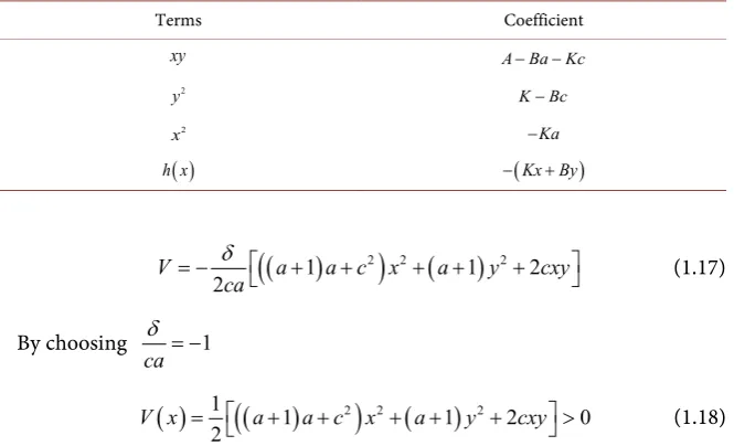
DOI: 10.4236/ojapps.2019.94017 203 Open Journal of Applied Sciences Table 1. A table showing terms and coefficients of Equation (1.12).

Terms Coefficient

xy A Ba Kc− −

2

y K Bc−

2

x −Ka

( )

h x −(Kx By+ )

(

)

(

₁ 2

)

2

(

₁

)

2 ₂

2

V a a c x a y cxy

ca

δ  

= − _ + + + + + _ (1.17)

By choosing 1

ca

2 ₂ ₀ 2

V x = _ a+ a c x+ + a+ y + cxy_> (1.18)

Using Equation (1.19) and the fact that V<0_{, the equilibrium point is}

asymptotically stable.

3.2. Stability Analysis of Periodic Solution of Duffing Equation

Using the Eigenvalue Approach

Considering the Duffing equation of the form (1.7), the first equivalent systems of (1.7) is given by

( )

2 ₂ 3

x y

y cy ax bx x h t

=

= − − − − +



 (1.19)

For the unforced case, Equation (1.19) is reduced to

2 ₂ 3

x y

y cy ax bx x

=

= − − − −



 (1.20)

At fixed points, x y= =0.

So that y=0 and _y__{= − −}_{ax bx}2₋₂_x3 ₌_{x ax bx}

(

_{− −} ₋₂_x2

)

₌_0.

Giving us x 0,x1 b ₄b2 8a

− + −

= = _and ₂ 2 8

4

b b a

x =− − − _which

corres-pond to

( )

0,0 ,

(

x1,0

)

and

(

x2,0

)

at fixed point. Analysis of the stability of

the fixed points can be done by linearizing Equation (1.20) which gives

(

₂ ₆ 2

)

x y

y cy a bx x x

=

= − − + +

 

   (1.21)

The matrix equation for (1.21) can be written as

(

2

)

0 1

2 6

x x

a bx x c

y y

 

   

=  

  _{− +} ₊ ₋  

 

  _ _ 

 

  (1.22)

(7)

(

2

)

0 1

2 6

a bx x c

λ

λ λ

−

 

 

− + + − − −

 

 

2 ₂ ₆ 2 ₀

c a bx x

λ +λ + + + + =λ

(

)

2 ₁ _c _g ₀

λ +λ + + = _(1.23)

(

₁

) (

₁

)

2 ₄ 2

2

)

1 1₂ 4g

λ = − +δ δ − _and

(

2

)

2 1₂ 4g

λ = − −δ δ − _where δ = +1 c_and

2

2 6

g a= + bx+ x

The coefficient of β shows that the Duffing equation is highly damped representing a hard spring. This hard spring is represented in Equation (1.21) where the coefficient of _x2_{is 6.}

At the origin, ( )0,0 1

(

2 _{4 .}

)

2 g

λ_± = − ±δ δ −

With δ =0_, _1,2 1

(

4 .

)

2 g

λ = ± −

For this, we consider the following cases:

1) When g=0, λ1,2 =0 and this implies that b x a, , are all zero;

2) When g>0, λ = ±1,2 i g which corresponds to critical points that are

centres for which stability is ensured;

3) When g<0, λ = ±1,2 g which corresponds to saddles giving rise to

in-stability [11].

With δ >0_,

(

2

)

1,2 1₂ 4 .g

λ = − ±δ δ −

For this, we consider the following cases: 1) When g=0, λ1,2 = −0, ;δ

2) When g>0_,

(

2

)

1,2

1 _{4 .}

2 g

λ = − ±δ δ −

For the discriminate, we have the following cases: When _{δ <}2 ₄_g_,

(

(

2

)

1,2

1 ₄

2 i g

λ = δ± δ + which leads to instability.

3) When _{δ +}2 ₄_g₌₀_,

( )

1,2 i g

λ

= ± which leads to centres and instability. Interestingly, for special case when c=0_{with no forcing term equation}

(1.20) becomes

x y= (1.25)

2 ₂ 3

y= − −ax bx − x (1.26)

The above can be integrated by quadrature, differentiating (1.25) and plugging in (1.26) gives

2 ₂ 3

x y = = − −ax bx − x (1.27)

Multiplying both sides by x gives

2 ₂ 3 ₀

xx axx bxx− −  − xx = (1.28)

Equation (1.28) can be written as

2 2 3 4

d 1 1 1 1 ₀

d 2t x 2ax 3bx 2x

 ₋ ₋ ₋ ₌

 

   (1.29)

So we have a variant of motion

2 2 3 4

1 1 1 1

2 2 3 2

h= x − ax − bx − x (1.30)

solving for _x_2_gives

2

2 d ₂ 2 2 3 4

d 3

x

x h ax bx x

t

 

=_ _ = + + +

 



2 3 4

d ₂ 2

d 3

x _{h ax} _bx _x

t = + + +

2 3 4

d d

2 2

3 t

t t

h ax bx x

= =

+ + +

∫

([35], p. 29)

Note that the invariant of motion h satisfies x h h x y

∂ ∂

= =

∂ ∂



 where

2 ₂ 3

h ax bx x y x

∂ ₌ ₊ ₊ ₌

∂  (1.31)

So the equation of Duffing oscillator are given by the Hamiltonian system h

x y

∂ =

∂

 and y h

x

∂ = −

∂

 ([35], p. 31)

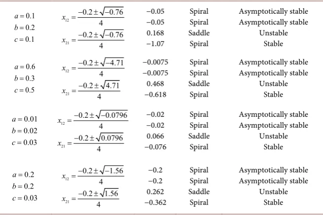
We consider the stability analysis of Duffing’s equation for different values of

(9)

[image:9.595.209.537.101.322.2]

DOI:10.4236/ojapps.2019.94017 206 Open Journal of Applied Sciences Table 2. The stability analysis and numerical solutions of duffing’s equation at different values a, b, c.

0.1 0.2 0.1 a b c = = = 12 21 0.2 0.76 4 0.2 0.76 4 x x − ± − = − ± − = −0.05 −0.05 0.168 −1.07 Spiral Spiral Saddle Spiral Asymptotically stable Asymptotically stable Unstable Stable 0.6 0.3 0.5 a b c = = = 12 21 0.2 4.71 4 0.2 4.71 4 x x − ± − = − ± = −0.0075 −0.0075 0.468 −0.618 Spiral Spiral Saddle Spiral Asymptotically stable Asymptotically stable Unstable Stable 0.01 0.02 0.03 a b c = = = 12 21 0.2 0.0796 4 0.2 0.0796 4 x x − ± − = − ± = −0.02 −0.02 0.066 −0.076 Spiral Spiral Saddle Spiral Asymptotically stable Asymptotically stable Unstable Stable 0.2 0.2 0.03 a b c = = = 12 21 0.2 1.56 4 0.2 1.56 4 x x − ± − = − ± = −0.2 −0.2 0.262 −0.362 Spiral Spiral Saddle Spiral Asymptotically stable Asymptotically stable Unstable Stable

Field work 2017.

3.3. Numerical Solution of Duffing’s Equation Using Mathcad

: 0.1 : 0.2 : 0.1

a = b = c =

0: 0 1: 150

t = t = _{Solution interval endpoints;} 0

: 1

ic _{=  } 

  Initial condition vector;

: 1500

N = Number of solution values on

[

t t0 1, .

]

(

)

_{( )}

1

_{( )}

2 3

0 0 0 1

, :

2 X D t X

a X b X X c X

 

=  

− ⋅ − ⋅ − ⋅ − ⋅

 

  Derivative function.

(

0 1

)

: , , , , .

S rkfixed ic t t N D=

0 :

T =S _{Independent variable values.} 1

1:

X =S _{Solution function values.}

2 2:

X =S _{Derivative function values.}

3.4. Stability Analysis of Duffing Equation under Oyesanya and

Nwamba (2013)

The unforced and damped cubic-quintic Duffing oscillator is given by

3 5 ₀

u+δu+αu+βu +µu = (1.32)

From Equation (1.32) we obtain the autonomous dynamical system

3 5

y u

y δu αu βu µu

= 



= − − − − _



  (1.33)

From the condition u=0 we obtain y=0 which gives us

3 5 ₀

u u u

(10)

Equation (1.34) can be written as

2 4 ₀

u_α β+ u +µu _= (1.35)

We obtain the roots of (1.35) as

2

0 0, 1,2,3,4 ₂1 4

u u β β µα

µ 

= = ± __− ± − __

Then the equation satisfied by the eigenvalues of our systems stability matrix is

2 ₃ _u2 ₅ _u4

λ +δλ= − −α β − µ (1.36)

where u denotes u u u1 2 3 and u4 or the u-coordinate of an equilibrium point.

Whether our eigenvalues will be complex, real or imaginary will be determined by the values of δ and _g₌₅_µ_u4₊₃_β_u2₊_α_{with = 0,}

_{( )}

1,2 1₂ 4g

λ ₌ _{± −} 

 .

For this we consider the following cases: 1) g=0_{: for this case} λ_1,2 =0.

This contradicts our assumption that det J≠0_{and it also implies that}

, ,

α β µ are all zero.

2) g>0: for this case λ = ±1,2 i g.

This corresponds to critical points that are centers for which stability is en-sured.

3) g<0: for this case λ = ±1,2 g which corresponds to saddles giving rise

to instability in (1.35) with δ >0,

2 1,2

1 ₄

2 g

λ = __− ±δ δ − __

Then considering the case below we have:

1) g=0: giving the values λ1,2= −0, δ which goes contrary to our

aassump-tion that det j≠0. It also implies that α β µ, , are all zero. 2) g>0: for this case

2

1,2 1₂ 4g

λ = __− ±δ δ − __

Considering the discriminant fot this case, we have three cases.

a) _{δ <}2 ₄_g _, 2

1,2 1₂ 4g

λ = __− ±δ δ − __ which corresponds to spirals and asymptotic stability.

b) The case _{δ >}2 ₄_g_{gives the values of the form}

1,2 1₂ p p, 0

λ = _− ±δ _ >

which corresponds to nodes resulting in asymptotic stability if δ > p and to saddles and consequently instability if δ < p.

c) _{δ =}2 ₄_g_gives

1,2 g

λ = ± _{. For this case we have saddles and hence}

insta-bility.

3) g<0 leads us to have 2

1,2 1₂ 4 .g

λ = __δ± δ − __

(11)

a) _{δ +}2 ₄_g_<₀_{: this case gives} 2

1,2 1₂ i 4g

λ = __δ ± δ − __ and we have spirals and consequently asymptotic stability.

b) _{δ +}2 ₄_g_>₀_gives

1,2 1₂ i Q Q , 0

λ = _δ± _ > _{and this leads us to the}

exis-tence of node and instability if δ > Q or saddles and instability if δ < Q.

c) _{δ +}2 ₄_g ₌₀_,

1,2 i g

λ

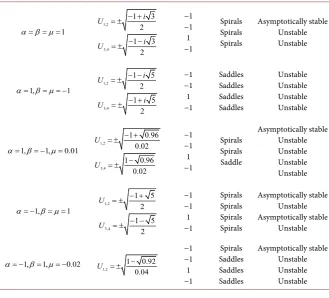
_{= ± } __{which yield centers and stability.}

We now consider the stability analysis of the dynamics for a few choices of

, ,

α β µ and δ by using employing Equations (1.35) and (1.36). These are il-lustrated in Table 3.

3.5. Stability Analysis of Torres (2004)

We consider the Duffing’s equation of the form

( )

, 0

x cx g t x+ + =

  (1.37)

with c>0_and g: 0,2

[

π

]

× →R R_{is a}_L1_{-caratheodory function such that}

the partial derivative gx exists and it is: 1

L-caratheodory. For a given 1≤ ≤ +∞p , let us define the set

(

)

2

( )

*

, p 0,2π : 0, 1 ₄ 2

p c p

c

a L a a k p

   

 

Ω = ∈ > < +  

   

 

[image:11.595.207.537.430.728.2]

with _{p k}*_, _{defined. Let}_ϕ_{be a 2π periodic solution of Equation (1.37), we}

Table 3. Stability analysis of the dynamics of the oscillator for few choices of parameter α,

β and μ.

1

α β µ= = = 1,2

3,4 1 3 2 1 3 2 i U i U − + = ± − − = ± −1 −1 1 −1 Spirals Spirals Spirals Asymptotically stable Unstable Unstable 1, 1

α= β µ= = − 1,2

3,4 1 5 2 1 5 2 i U i U − − = ± − + = ± −1 −1 1 −1 Saddles Saddles Saddles Saddles Unstable Unstable Unstable Unstable

1, 1, 0.01

α= β= − µ= 1,2

3,4 1 0.96 0.02 1 0.96 0.02 U U − + = ± − = ± −1 −1 1 −1 Spirals Spirals Saddle Asymptotically stable Unstable Unstable Unstable Unstable 1, 1

α= − β µ= = 1,2

3,4 1 5 2 1 5 2 U U − + = ± − − = ± −1 −1 1 −1 Spirals Spirals Spirals Spirals Asymptotically stable Unstable Asymptotically stable Unstable

1, 1, 0.02

α= − β= µ= −

1,2

1 0.92 0.04

U = ± −

(12)

assume that a∈ Ωp c, exists such that

( )

(

,

)

( )

x

g tϕ x <a t for a.e t∈

[

0,2π

]

_(1.38)

For such an a, the operator L as defined in maximum principle is inversely positive. By defining the operator.

[

]

1

(

)

: 0,2π 0,2π

1

γ ϕ ≤ .

4. Discussion

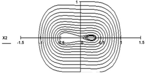
Figure 1 is the MATCAD showing the behavior of the Duffing’s equation when

0.1, 0.2

a= b= _and c=0.1_{is periodic. We observe asymptotically stable at}

both saddle and spiral point i.e. _−0.2± −₄ 0.76 ,0_

  which are three equilibrium

points observed. This situation is seen in Duffing’s equation.

Figure 2 shows the dynamics of Duffing’s equation when

0.6, 0.3, 0.5

a= b= c= . We observed asymptotically stable at spiral point i.e.

0.3 _{4.71 ,0} 4

− ± − 

 

 . This shows that the phase is revolving round it. At (0.468)

the point was saddle showing that it is unstable.

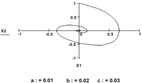
Figure 3: the MATCAD shows the dynamics of the Duffing’s equation when

0.01, 0.02, 0.03

a= b= c= . Three equilibrium points was observed. Saddles were obtained at

(

−0.02,0.066

)

showing that the phases are toward the origin.

Figure 4: the MATCAD were obtained for the values of

0.2, 0.2, 0.03

a= − b= c= . In this case it is important to note that the phase line tend to converge toward the equilibrium points.

Figure 5: The trajectory profile of Duffing’s equation were obtained for the values a= −0.2,b=0.2,c=0.03. In this case, there is an increase in oscillation which is as a result of decrease in the damping coefficient. That is decrease in damping leads to increase in oscillation.

Figure 6: The phase portrait of Duffing’s equation was obtained. We observed that the phase line was depicting a center of non-stable node.

Figure 7: The trajectory profile of Duffing’s equation were obtained for the values a=0.6,b=0.3,c=0.5_{. In this case, there is a decrease in the maximum}

displacement from the origin which leads to decrease in oscillation. The decrease in oscillation is as a result of increase in the damping coefficient. That is increase in damping leads to decrease in oscillation.

Figure 8: In this case, the phase portrait was depicting the center as an unsta-ble node.

5. Conclusion

(13)

[image:13.595.233.518.72.190.2] [image:13.595.256.495.229.357.2]

DOI:10.4236/ojapps.2019.94017 210 Open Journal of Applied Sciences Figure 1. Trajectory profile of Duffing equation for values a=0.1,b=0.2,c=0.1_.

Figure 2. Phase portrait of Duffing’s equation showing asymptotic stability of solution as a spiral sink.

Figure 3. Trajectory profile of Duffing equation for values 0.6, 0.3, 0.5

a= b= c= .

[image:13.595.258.493.405.516.2] [image:13.595.259.490.558.693.2]

(14)

[image:14.595.259.492.72.171.2]

DOI: 10.4236/ojapps.2019.94017 211 Open Journal of Applied Sciences Figure 5. Oscillatory profile of Duffing equation for parameters

0.2, 0.2, 0.03

[image:14.595.253.493.220.370.2]

a= − b= c= .

Figure 6. Phase portrait of Duffing’s equation depicting a centre of a non-stable node.

Figure 7. Oscillatory profile of Duffing equation for values 0.6, 0.3, 0.5

a= b= c= .

[image:14.595.257.490.418.536.2] [image:14.595.254.490.588.709.2]

(15)

method and Matcad has yielded successful results. We discovered that global stability of periodic solution was achieved through the construction of a suitable and complete Lyapunov function for the hard spring system using Cartwright method. From the above tables discussed and outlined, we could see that the stability behaviours of the solutions are similar despite the different methods. Our technique showed superiority above others because stability is a property of the equilibrium point and of the system.

Conflicts of Interest

The authors declare no conflicts of interest regarding the publication of this paper.

References

[1] Bender, C.M. and Orszag, S.A. (1999) Advanced Mathematical Method for Scien-tists and Engineers Asymptotic Methods and Perturbation Theory. Springer, New York, 545-551.

[2] Zeeman, E. (1976) Duffing Equation in Brain Modelling. Bulletin Institute of Ma-thematics and Its Applications, 12, 207-214.

[3] Oyesanya, M.O. (2008) Duffing Oscillator as Model for Predicting Earthquake Oc-currence I. Journal of Nigerian Association of Mathematical Physics, 12, 133-142. [4] Wang, G., Zheng, W. and He, S. (2002) Estimation of Amplitude and Phase of a

Weak Signal by Using the Property of Sensitive Dependence on Initial Condition of a Non-Linear Oscillator. Signal Processing, 82, 103-115.

https://doi.org/10.1016/S0165-1684(01)00166-9

[5] Yang, L. and Li, Y.K. (2014) Existence and Global Exponential Stability of Almost Periodic Solution for a Class of Delay Duffing Equation on Time Scale. Abstract and Applied Analysis, 2014, Article ID: 857161.

https://doi.org/10.1155/2014/857161

[6] Bhatti, M. and Lara M. (2008) Periodic Solutions of the Duffing Equation. Birkhäu-ser Verlag, Bassel, Switzerland.

[7] Sani, G. and Allain, H. (1989) N-Cyclic Function and Multiple Subharmonic Solu-tions of Duffing Equation.

[8] Ortega, R. (1994) Some Application of Topological Degree to Stability Theory in Topological Methods in Differential Equation and Inclusion. Journal of London Mathematical Society, 42, 505-516.

[9] Njoku, F.I. and Omari, P. (2003) Stability Properties of Periodic Solutions of a Duffing Equation in the Presence of Lower and Upper Solutions. Applied Mathe-matics and Computation, 135, 471-490.

https://doi.org/10.1016/S0096-3003(02)00062-0

[10] Torres, P.J. (2004) Existence and Stability of Periodic Solutions of a Duffing Equa-tion by Using a New Maximum Principle. Mediterranean Journal of Mathematics, 1, 470-486. https://doi.org/10.1007/s00009-004-0025-3

[11] Oyesanya, M.O. and Nwamba, J.I. (2013) Stability Analysis of Damped Cu-bic-Quintic Duffing Oscillator. World Journal of Mechanics, 3, 43-57.

https://doi.org/10.4236/wjm.2013.31003

(16)

Differen-DOI: 10.4236/ojapps.2019.94017 213 Open Journal of Applied Sciences tial Equations. Nigeria Journal of Science Association, 1, 5-10.

[13] Ezeilo, J.O.C. (1963) An Extension of a Property of the Phase Space Trajectories of a Third Order Differential Equation. Annali di Matematica Pura ed Applicata, 63, 387-397. https://doi.org/10.1007/BF02412186

[14] Afuwape, A.U. (1983) Ultimate Boundedness Result for a Certain System of Third Order Non-Linear Differential Equation. Journal of Mathematical Analysis and Ap-plication, 97, 140-150. https://doi.org/10.1016/0022-247X(83)90243-3

[15] Afuwape, A.U. (1983) Uniform Utimate Boundedness Result for Some Third Order Nonlinear Differential Equation. KTP, Trieste, preprint IC/90/405.

[16] Ogundare, S.A. (2009) Qualitative and Quantitative Properties of Solution of Ordi-nary Differential Equations. Ph.D. Thesis, University of Forte Hare, Alice, South Africa, 48-63.

[17] Nayfeh, A.H. and Mook, D.T. (1979) Nonlinear Oscillation. Wiley Publication, New York.

[18] Thomsen, J.J. (2003) Vibration and Stability. Advanced Theory, Analysis and Tools. Springer, Toronto, London, 273-281. https://doi.org/10.1007/978-3-662-10793-5 [19] Seyranian, A.P. and Wang, Y. (2011) On Stability of Periodic Solution of Duffing

Equation. Journal of National Academy of Science of Armenia, 111, 211-232. [20] Moon, F.C. and Holmes, P.J. (1979) Chaotic Oscillators: Theory and Applications.

Journal of Sound and Vibration, 65, 275-296.

[21] Haung, J.H., Su, R., Khali, H.K. and Chen, S.H. (2009) Computers and Studies. In-ternational Journal of Mathematical Analysis, 87, 1624-1630.

[22] El-Bassiouny, A.F. and Abadel-Khalik, A. (2010) Evolution Equation. Physica Scripta, 81, 56-62.

[23] Cartwright, M.L. (1956) On the Stability of Solution of Certain Differential Equa-tion of the Fourth Order. The Quarterly Journal of Mechanics and Applied Mathe-matics, 9, 185-194. https://doi.org/10.1093/qjmam/9.2.185

[24] Tiryaki, A. and Tunc, C. (1995) Construction of Lyapunov Function for Certain Fourth-Order Autonomous Differential Equation. Indian Journal of Pure Applica-tion of Mathematics, 26, 225-232.

[25] Delves, L.M. and Mohamed, J.L. (1985) Computer Methods for Integral Equations. Cambridge University Press, New York, 376.

https://doi.org/10.1017/CBO9780511569609

[26] Hairer, Z., Ernst, J., Wanner, D. and Gerhard, G. (1991) Solving Ordinary Differen-tial Equation. In: Springer Series in Computational Mathematics, Vol. 73, Sprin-ger-Verlag, Berlin, 273-289.

[27] Atkinson, F.A. (1955) On Second Order Non-Linear Oscillation. Pacific Journal of Mathematics, 5, 643-647. https://doi.org/10.2140/pjm.1955.5.643

[28] Boyd, P.J. (2000) Chebychev and Fourier Spectral Method Edition. Dover Publica-tion Inc., New York, 360.

[29] Jordan, D.W. and Smith, P. (1977) Nonlinear Analysis and Differential Equations. Clavendon Press, Oxford.

[30] Thompson, J.M.T. and Stewart, H.B. (1986) Nonlinear Dynamics and Chaos. John Wiley & Sons, New York.

[31] Puu, T. (2000) Attractors, Bifurcations and Chaos. Non-Linear Phenomena in Eco-nomics. 2nd Edition, Springer Verlag, Berlin Heidelberg, 465-469.

(17)

DOI:10.4236/ojapps.2019.94017 214 Open Journal of Applied Sciences [32] Ueda, Y. (2000) Randomly Transitional Phenomena in the System Governed by

Duffing’s Equation. Journal of Statistical Physics, 20, 181-196. https://doi.org/10.1007/BF01011512

[33] Zhang, W.B. (2005) Differential Equations, Bifurcations and Chaos in Economics. 4th Edition, World Scientific Publishing, Hackensack, NJ, 231-243.

https://doi.org/10.1142/5827

[34] Ezeilo, J.O.C and Ogbu, H.M. (2009) Construction of Lyapunov Type of Functions for Some Third Order Differential Equation by Method of Integration. Journal of Science Teaching Association of Nigeria, 45, 59-63.

[35] Wiggins, S.S. (1990) The Geometrical Point of View of Dynamical Systems: Back-ground Material, Poincaré Maps, and Examples. In: Introduction to Applied Non-linear Dynamical Systems and Chaos, Springer Verlag, New York, 5-192.