Optimal Ordering Policy for Deteriorating Items with Limited Storage Capacity under Two Level Trade Credit Linked to Order Quantity by a Discounted Cash Flow Analysis

(1)

ISSN Online: 2329-3292 ISSN Print: 2329-3284

DOI: 10.4236/ojbm.2019.72063 Apr. 24, 2019 919 Open Journal of Business and Management

Optimal Ordering Policy for Deteriorating

Items with Limited Storage Capacity under

Two-Level Trade Credit Linked to Order

Quantity by a Discounted Cash-Flow Analysis

Hui-Ling Yang

Department of Computer Science and Information Engineering, Hungkuang University, Taiwan

Abstract

Nowadays, the supplier often provides cash discount or permissible delay in payments to its retailers, if the order quantity attains a certain amount. Like-wise, the retailer also provides a downstream trade credit period to his cus-tomers. In practice, as the supplier provides price discounts for bulk purchas-es, the retailer may purchase more goods than can be stored in its owned warehouse and store the excess quantities in a rented warehouse. Thus, a two-warehouse inventory model is needed to be considered. Further, the cost is usually affected by the present value of time and products deteriorate as time increases. Therefore, this paper develops a supplier-retailer-customer chain inventory model in which 1) two-level trade credit linked to order quantity is considered; 2) storage capacity is limited; 3) the effect of inflation and time value of money by a discounted cash-flow analysis is taken into ac-count. The demand rate is linearly increasing with time and the deterioration rate is constant. Based on the viewpoint of cost minimization, the objective is to find the optimal replenishment cycle and order quantity to keep the present value of the total relevant cost per unit time as minimum as possible. The research shows that in each case discussed, the optimal solution for each case exists uniquely. Finally, numerical examples are provided for illustration and some managerial insights based on the numerical results are also pre-sented.

Keywords

Deterioration, Storage Capacity, Trade Credit, Order Quantity, Discounted Cash Flow

How to cite this paper: Yang, H.-L. (2019) Optimal Ordering Policy for Deteriorating Items with Limited Storage Capacity under Two-Level Trade Credit Linked to Order Quantity by a Discounted Cash-Flow Analy-sis. Open Journal of Business and Man-agement, 7, 919-940.

https://doi.org/10.4236/ojbm.2019.72063 Received: March 19, 2019

Accepted: April 21, 2019 Published: April 24, 2019

(2)

DOI: 10.4236/ojbm.2019.72063 920 Open Journal of Business and Management

1. Introduction

In the classical EOQ model, the supplier often prefers to offer his customers a delay period for payment to attract new customers and promote more sales, es-pecially in the present of economic depression circumstances. Usually, there is no interest charge if the outstanding amount is paid within this permissible de-lay period. However, if the payment is unpaid in full by the end of the permissi-ble delay period, interest is charged on the outstanding amount. On the other hand, the policy of granting credit terms adds an additional cost to the supplier as well as an additional dimension of default risk. The literature reviews are de-scribed as the following subsections.

1.1. Papers Related with Permissible Delay in Payment

or Two-Level Trade Credit

Goyal [1] developed an EOQ model under the conditions of a permissible delay in payments, and ignored the difference between the selling price and the pur-chase cost. Shah [2] considered a stochastic inventory model when delays in payments are permissible. Aggarwal and Jaggi [3] extended Goyal’s model to consider the deteriorating items. Jamal et al. [4] further generalized Aggarwal and Jaggi’s model to allow for shortages. Concurrently, Hwang and Shinn [5] added the pricing strategy to the model, and developed the optimal price and lot-sizing for a retailer under the condition of a permissible delay in payments. Chang and Dye [6] proposed an inventory model for Weibull distribution dete-riorating items with partial backlogging and permissible delay in payments. Teng et al. [7] provided an economic order quantity model with trade credit fi-nancing for non-decreasing demand. Other related research articles can be found in Teng [8], Teng et al. [9], Hsieh et al. [10] and their references.

The aforementioned models assumed that the supplier offers the retailer a permissible delay period in payment (i.e., an upstream trade credit). Sometimes, the retailers also do such a way to their customers (i.e., a downstream trade credit). It is a so-called two-level trade credit policy. Huang [11] proposed an optimal retailer’s ordering policies in the EOQ model under trade credit financing. Ouyang et al. [12] proposed an EOQ model for deteriorating items under trade credit. Teng and Goyal [13] provided an optimal ordering policy for a retailer in a supply chain with up-stream and down-stream trade credits. Min et al. [14] proposed an inventory model for deteriorating items under stock-dependent de-mand and two-level trade credit. Lately, Rameswari and Uthayakumar [15] pro-vided an integrated inventory model for deteriorating items with price-dependent demand under two-level trade credit policy.

1.2. Papers Related with Permissible Delay in Payment

or Two-Level Trade Credit Linked to Order Quantity

(3)

DOI: 10.4236/ojbm.2019.72063 921 Open Journal of Business and Management et al. [16] developed an EOQ model for deteriorating items under supplier cre-dits linked to ordering quantity. Chung and Liao [17] provided lot-sizing deci-sions under trade credit depending on the ordering quantity. Jaggi et al. [18] proposed retailer’s optimal replenishment decisions with credit-linked demand under permissible delay in payments.

In order to encourage more sales, the supplier often offers the retailer with conditional permissible delay period as the retailer orders more than a prede-termined quantity. Kreng and Tan [19] proposed an inventory model under two levels of trade credit depending on the order quantity. Teng et al. [20] provided an inventory model for deteriorating demand under two levels of trade credit linked to order quantity. Recently, Sash and Cárdenas-Barrón [21] provided an inventory model which is a retailer’s decision for ordering and credit policies with deteriorating items when a supplier offers order-linked credit or cash dis-count. Ting [22] gives some comments on the EOQ model for deteriorating items with conditional trade credit linked to order quantity. Many related re-search articles can be found in their references.

1.3. Papers Related with Trade Credit and Limited Storage

Capacity or Discounted Cash Flow Analysis

As the suppliers provide price discounts for bulk purchases, the retailer may purchase more goods than can be stored in its owned warehouse and store the excess quantities in a rented warehouse. Chung and Huang [23] proposed the inventory model for deteriorating items with limited storage capacity under permissible delay in payments. Huang [24] proposed an inventory model under two levels of trade credit and limited storage space without derivatives. Chung and Huang [25] provided an optimal retailer’s ordering policies for deteriorating items with limited storage capacity under trade credit financing. Ouyang et al. [26] proposed an EOQ model with limited storage capacity under trade credits.. Recently, Lin et al. [27] provided an integrated inventory model for two-stage deterioration under trade credit and variable capacity utilization.

In reality, due to today’s competitive markets, the relevant costs involved in the inventory model are affected by the effect of inflation and time value of money. Thus, to consider not only the opportunity loss (i.e., time value of mon-ey) of trade credit, but also on all relevant costs is necessary. Chen and Teng [28] provided an inventory and credit decisions for time-varying deteriorating items with up-stream and down-stream trade credit financing by discounted cash flow analysis. Wu et al. [29] proposed inventory models for deteriorating items with maximum lifetime under downstream partial trade credit to credit-risk custom-ers by discounted cash-flow analysis. Li et al. [30] provided a pricing and lot-sizing policies for perishable products with advance-cash-credit payments by a discounted cash-flow analysis.

(4)

of inflation and time value of money by a discounted cash-flow analysis is in-corporated. The demand rate is linearly increasing with time and the deteriora-tion rate is constant. If the order quantity exceeds the predetermined quantity or the capacity of own-warehouse, then an upstream trade credit period is permit-ted or it is necessary to rent a warehouse to store the excessive items. That is, a generalized deteriorating inventory model with limited storage capacity under two levels of trade credit linked to order quantity and by a discounted cash-flow analysis is considered. As a result, this paper is a general framework that in-cludes numerous previous models as special cases, such as Chang et al. [16], Chung and Liao [17], Teng et al. [20] and others. Based on the viewpoint of cost minimization, the objective is to find the optimal replenishment cycle and order quantity to keep the present value of the total relevant cost per unit time as minimum as possible. Numerical examples are provided for illustration and some managerial insights are presented.

The remainder of the paper is structured as follows. Section 2 introduces the as-sumptions and notation needed to develop the proposed inventory model. Section 3 formulates the model. Section 4 discusses some theoretical results and provides an algorithm to find the optimal solutions. Section 5 provides numerical examples to illustrate the proposed model. Section 6 concludes the results and presents some managerial insights. Further, provides some future research directions.

2. Assumptions and Notation

In this research, the mathematical models proposed are based on the following assumptions:

1) Lead time is zero and replenishment is instantaneous. 2) Shortages are not allowed.

3) The own warehouse has a limited capacity W and the rented warehouse has unlimited capacity.

4) A constant fraction of the on-hand inventory deteriorates per unit of time and there is no repair or replacement of the deteriorated inventory (i.e., the sal-vage value of a deteriorating item is zero). Without loss of generality, assuming that the deterioration rate in both own warehouse (OW) and rented warehouse (RW) is the same.

5) If the order quantity is larger than the capacity of own warehouse, then the retailer will rent a warehouse to store the excessive items. For economic reasons, the goods of RW are consumed and cleared before OW.

6) The inventory costs (including holding cost and deterioration cost) in RW are higher than those in OW.

7) If the order quantity is larger than the predetermined order quantity, then the delay in payment offered by supplier is permitted, otherwise, the retailer must pay immediately as the items received.

(5)

retailer needs not to pay any interest charged by the supplier. If not, the retailer needs to pay the interest charged on the items in stock to the supplier.

10) The retailer can accumulate revenue and earn interest after his customers pay for the amount until the end of the trade credit period offered by the supplier.

In addition, the following notation is used throughout this paper.

( )

f t = the demand rate at time t, we here assume that f t

( )

is linear time dependent, i.e., f t

( )

= +a bt_.

W = the capacity of owned warehouse (OW). Q = the order quantity.

d

Q = the predetermined order quantity at which the delay is permitted by the supplier.

d

T = the time interval that Qd units are depleted to zero due to both de-mand and deterioration.

a

T = the time at which the inventory level reaches W units due to both

de-mand and deterioration where a 0, if _{0, if} Q W T

Q W

= ≤



 > >

 .

w

T = the time interval that W units are depleted to zero due to both demand and deterioration.

M = the retailer’s trade credit period offered by supplier in years. N = the customer’s trade credit period offered by retailer in years. T = the length of replenishment cycle in years, where T T T= a+ w. r = the annual interest rate per year.

θ_{= the deterioration rate, where} 0< <θ 1_. A = the replenishment cost per order.

h = the holding cost per unit per unit time in OW excluding interest charge. k = the holding cost per unit per unit time in RW excluding interest charge. From Assumption 5, we have k h> .

c = the unit purchasing cost. e

I = the interest earned per dollar per unit time per year by the retailer.

p

I = the interest paid per dollar per unit time per year by the retailer.

( )

I t = the inventory level at time t.

( )

ij

TC T = the present value of the annual total relevant cost per unit time, which is a function of T, where i=1,2,3,4, j=1,2_.

*

T = the optimal replenishment cycle time of TC Tij

( )

, i=1,2,3,4, 1,2

j= _.

*

Q = the optimal order quantity.

3. Research Models

For the model, the inventory depletes due to the combined effect of demand and deterioration. The inventory level at time t is governed by the following differen-tial equations:

( )

_{( )}

d

, 0 d

I t

f t I t t T

(6)

with the boundary condition I T

( )

=0_{The solutions to (1) is}

( )

e t Teu

( )

d , 0 t

I t ₌ −θ θ f u u _{≤ ≤}t T

∫

(2)

Thus, the order quantity for each cycle is

( )

0 ₀Tet

( )

d

Q I₌ ₌ θ f t t

∫

.

(3) From Equation (3), we can obtain the time interval Td, Ta and Tw by us-ing the followus-ing equations:

( )

0 e d

d T _t d

Q ₌ θ f t t

∫

(4)

( )

e d a

T _t T

W₌ θ f t t

∫

(5) and

( )

0 e d , if

a T _t

Q W₋ ₌ θ f t t Q W_>

∫

(6)

respectively. Therefore, the profit of the inventory system consists of the follow-ing components.

1) The ordering cost is A.

2) If Q W≤ _{, then the inventory holding cost in RW and OW are}

0 HR

C = _,

and

( )

_{( )}

0e d 0e e d d

T _rt T _{r t} T _u

HO _t

C ₌h − I t t h₌ − +θ θ f u u t

∫

.

(7)

If Q W> _{, then the inventory holding cost in RW and OW are}

( )

_{( )}

0 e d 0 e e d d 0 e d

a a a a

T _rt T _{r t} T _u T _rt

HR _t

C ₌k − _I t W t k₋ _ ₌  − +θ θ f u u t W₋ − t

  __ __

∫

and

( ) ( )

_{( )}

0 e d e e d d

a

T _{r t} T _{r t} T _u

HO _T _t

C ₌h W − +θ t₊ − +θ θ f u u t

 



∫

.

(8)

3) The deteriorating cost is ₀Te rt

( )

d d

C ₌

θ

c − I t t

∫

.

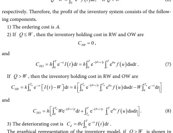
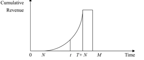
[image:6.595.203.542.284.545.2]

The graphical representation of the inventory model, if Q W> _{is shown in}

Figure 1.

3.1. Q Q

<

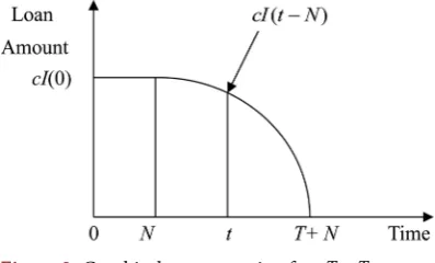
_d

In this case, the retailer’s order quantity is less than Qd. Hence, the permissible delay in payment is not allowed (i.e., M = 0). Meanwhile, the retailer offers a permissible delay of N to its buyers. Consequently, the retailer must fiancé all items ordered at time 0, and start to payoff the loan after time N. For details, please see Figure 2. Thus, the interest paid by the retailer is

( )

₍

₎

( )

( )( )

_{( )}

0

0 0

e 0 d e d

e e d d e e d d

N _rt T N _{r t N}

p _N

N _rt T _u T N _{r t N} T _u

p _N _{t N}

cI I t I t N t

cI θ f u u t θ θ f u u t

+ ₋ ₋ −

+ _{− +} ₋ −

−

 ₊ ₋ 

 

 

 

= __ + __

∫

(7)

[image:7.595.246.505.67.247.2]

[image:7.595.274.473.278.398.2]

Figure 1. Graphical representation of the inventory Model, if Q W> .

Figure 2. Graphical representation for T T< d.

Based on whether the order quantity is larger than the capacity of own ware-house or not, there are two sub-case: i) Q W≤ ii) Q W> .

Hence, the present value of the retailer’s annual total relevant cost per unit time is

( )

{

(

)

( )

_{( )}

( )

( )( )

_{( )}

}

11 ₀

0 0

e e d d

e e d d , if

T _{r t} T _u t N _rt T _u p

T N _{r t N} T _u

N t N

TC T A h c f u u t

cI f u u t

f u u t T Q W

θ θ

θ

θ θ

θ − +

−

+ _{− +} ₋ −

= + +

 + _



+ _ ≤

∫

(10)

( )

{

( )

_{( )}

( ) ( )

_{( )}

( )

_{( )}

( )

( )( )

_{( )}

}

12 ₀

0

0 0

e e d

i d

e d e e d d

e e d d e d

e e d d

e e d d , f

a

a a a

T _{r t} T _u t

T _{r t} T _{r t} T _u

T t

T _{r t} T _u T _rt

t N _rt T _u p

T N _{r t N} T _u

N t N

TC T A c f u u t

h W t f u u t

k f u u t W t

cI f u u t

f u u t T Q W

θ θ

θ θ θ

θ θ

θ

θ θ

θ − +

− + − +

− + −

−

+ _{− +} ₋ −

= +

 

+ _ + _

 

 

+ _ − _

 

 + _



+ _ >

∫

(11)

3.2. Q Q

≥

_d

(8)

pay-DOI: 10.4236/ojbm.2019.72063 926 Open Journal of Business and Management

ment time T + N, the retailer has three possible choices on its replenishment cycle time T: 1) 0<M N< ₂₎ 0<N M≤ _and M T N≤ + ₃₎ 0<N M≤

and M T N> + .

3.2.1. The Case of 0<M N<

Since M N< _{, there is no interest earned for the retailer. In addition, the}

retail-er has to finance all items ordretail-ered aftretail-er time M at an interest charged Ip per

dollar per year, and start to payoff the loan after time N as shown in Figure 3. Consequently, the interest charged is given by

( )

_{( )}

( )

₍

₎

( )

_{( )}

( )( )

_{( )}

0

e 0 d e d

e e d d e e d d

N _{r t M} T N _{r t N}

p _M _N

N _{r t M} T _u T N _{r t N} T _u

p _M _N _{t N}

cI I t I t N t

cI θ f u u t θ θ f u u t

+

− − − −

+

− − − + −

−

 ₊ ₋ 

 

 

 

= __ + __

∫

(12)

In the same way, based on whether the order quantity is larger than the capac-ity of own warehouse or not, there are two sub-case: i) Q W≤ _ii) Q W> _.

Hence, the present value of the retailer’s annual total relevant cost per unit time is

( )

{

(

)

( )

_{( )}

( )

_{( )}

( )( )

_{( )}

}

21 ₀

0

e e d d

e

if

e d d

e e d d ,

T _{r t} T _u t N _{r t M} T _u p _M

T N _{r t N} T _u

N t N

cI f u u t

f u u t T Q W

θ θ

θ

θ θ

θ − +

− −

+ _{− +} ₋ −

= + +

 + _



+ _ ≤

∫

(13)

( )

{

( )

_{( )}

( ) ( )

_{( )}

( )

_{( )}

( )

_{( )}

( )( )

_{( )}

}

22 ₀

0

0 0

0

e e d d

e d e e d d

e e d d e d

e e d d

e e d d , if

a

a a a

T _{r t} T _u t

T _{r t} T _{r t} T _u

T t

T _{r t} T _u T _rt

t N _{r t M} T _u p _M

T N _{r t N} T _u

N t N

h W t f u u t

k f u u t W t

cI f u u t

f u u t T Q W

θ θ

θ θ θ

θ θ

θ

θ θ

θ − +

− + − +

− + −

− −

+ _{− +} ₋

−

= +

 

+ _ + _

 

 

+ __ − __

 + _



+ _ >

∫

(14)

[image:8.595.253.497.586.709.2]

Note that Equations (10) and (11) are special cases of Equations (13) and (14) in which M = 0.

(9)

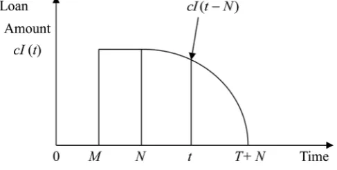
3.2.2. The Case of 0< N M≤ and M T N≤ +

When M T N≤ + _{, the retailer cannot receive the last payment before the}

per-missible delay time M. As a result, the retailer must finance all items sold after time (M N− _{) at time}_M_{, and pay off the loan until}_T₊_N_{at an interest rate of}

p

I per dollar per year as shown in Figure 4. Therefore, the interest paid is given by

( )

₍

₎

( )( )

_{( )}

e d e e d d

T N _{r t M} T N _{r t M} T _u

p _M p _M _{t M}

cI + − − I t M t cI + − +θ − θ f u u t

−

− =

∫

. (15)

On the other hand, the retailer starts selling products at time 0, and receiving the money at time N. Consequently, the retailer accumulates sales revenue in an account that earns Ie per dollar per year starting from N through M as shown in Figure 4. Therefore, the interest earned is given by

( )

₍

₎

e d d

M _{r t N} t

e N N

pI − − f u N u t₋

∫

.

(16) Likewise, based on whether the order quantity is larger than the capacity of own warehouse or not, there are two sub-case: i) Q W≤ ii) Q W> .

As a result, the present value of the retailer’s annual total relevant cost per unit time is

( )

{

(

)

( )

_{( )}

( )( )

_{( )}

( )

₍

₎

}

31 ₀e

if

e d d

e e d d

e d d ,

T _{r t} T _u t T N _{r t M} T _u

p M t M

M _{r t N} t

e N N

cI f u u t

pI f u N u t T Q W

θ θ

θ − +

+ _{− +} ₋ −

− −

= + +

+

− − ≤

∫

(17)

( )

{

( )

_{( )}

( ) ( )

_{( )}

( )

_{( )}

( )( )

_{( )}

( )

₍

₎

}

32 ₀

0

0 0

e e d d

e d e e d d

e e d d e d

e e d d

e d d , fi

a

a a a

T _{r t} T _u t

T _{r t} T _{r t} T _u

T t

T _{r t} T _u T _rt

t

T N _{r t M} T _u

p M t M

M _{r t N} t

e N N

h W t f u u t

k f u u t W t

cI f u u t

pI f u N u t T Q W

θ θ

θ θ θ

θ θ

θ − +

− + − +

− + −

+ _{− +} ₋ −

− −

= +

 

+ _ + _

 

 

+ _ − _

 

+

− − >

∫

(18)

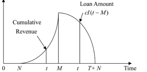
3.2.3. The Case of 0< N M≤ and M T N> +

[image:9.595.257.505.587.708.2]

Since the order quantity is larger than or equal to Qd, the retailer receives the

(10)

permissible delay in payment. If M T N> + _{, then the retailer receives all}

pay-ments from its customers by the time T + N which is before the permissible de-lay time M. Hence, the retailer has the money to pay the supplier at time M, and does not have the interest charges. In the meantime, the retailer receives the revenue and deposits into a bank to earn interest as shown in Figure 5. The in-terest earned by the retailer is

( )

₍

₎

( )

_{( )}

0

e d d e d d

T N _{r t N} t M _{r t T N} T

e _N _N _{T N}

pI + − − f u N u t − − − f u u t

+

 ₋ ₊ 

 



∫

. (19)

Similarly, based on whether the order quantity is larger than the capacity of own warehouse or not, there are two sub-case: i) Q W≤ _ii) Q W> _.

Therefore, the present value of the retailer’s annual total relevant cost per unit time is

( )

{

(

)

( )

_{( )}

( )

₍

₎

( )

_{( )}

}

41 ₀

0

e e d d

e d d

e d d , if

T _{r t} T _u t T N _{r t N} t

e _N _N

M r t T N T T N

pI f u N u t

f u u t T Q W

θ θ

θ − +

+ ₋ ₋

− − − +

= + +



− _ −



+ _ ≤

∫

(20)

( )

{

( )

_{( )}

( ) ( )

_{( )}

( )

_{( )}

( )

₍

₎

( )

_{( )}

}

42 ₀

0

0 0

0

e e d d

e d e e d d

e e d d e d

e d d

e d d , fi

a

a a a

T _{r t} T _u t

T _{r t} T _{r t} T _u

T t

T _{r t} T _u T _rt

t T N _{r t N} t

e _N _N

M _{r t T N} T T N

h W t f u u t

k f u u t W t

pI f u N u t

f u u t T Q W

θ θ

θ θ θ

θ θ

θ − +

− + − +

− + −

+ ₋ ₋

− − −

+

= +

 

+ _ + _

 

 

+ _ − _

 



− _ −



+ _ >

∫

(21)

4. Theoretical Results

In order to find the optimal solution of each case, we derive the theoretical re-sults in the following two ways: i) Q W≤ _ii) Q W> _.

4.1. The Case of Order Quantity Is Not Greater than the Capacity of

Own-Warehouse (

i.e.

,

Q W

≤

)

[image:10.595.245.518.595.709.2]

In this sub-section, we discuss each case shown in Section 3 as the order quantity

(11)

is not greater than the capacity of own-warehouse. To minimize the present value of the total relevant cost, it is necessary to calculate the first and second order de-rivatives of TC Ti1

( )

, i=1,2,3,4, with respect to T, and let dTC Ti1

( )

dT =0. We have the following results.

(

)

(

)

( )

11

d _e 1 e

d

1 e ₀

r T T

p rN

p

TC _{a bT} _h _{c cI}

T r

cI TC T

r θ θ _θ θ − + −    −   = +  + + _ ₊ _          −   +  −  =    (22)

(

)

(

)

( )

(

)

(

)

( ) 11 2 11 2 d ₀ d d d 1 e e

1 e _e _e ₀

TC T r T T p rN r T T p p TC T

a bT b h c cI

r

cI a bT h c cI T

r θ θ θ θ θ θ θ θ = − + − − +    ₋   =  + +   + + _ ₊ _          −  

+ _ __+ + + + _ >

   (23)

(

)

(

)

( ) ( ) 21 21

d _e 1 e

d

1 e ₀

r T T

p

r N M

p

TC _{a bT} _h _{c cI}

T r

cI TC T

r θ θ _θ θ − + − −    −   = +  + + _ _ +          −   + _ _−  =     (24)

(

)

(

)

( ) ( )

(

)

(

)

( ) 21 2 21 2 _d 0 d d d 1 e e

1 e _e _e ₀

TC T

r T T

p

r N M

r T T

p p

TC T

a bT b h c cI

r

cI a bT h c cI T

r θ θ θ θ θ θ θ θ = − + − − − +    −   = _ + +  _ + + _ _ +          −  

+ _ _+ + + +  >

    (25)

(

) (

)

( ) ( )( ) ( )( )

_{( )}

31 31

d _e 1 e 1 e

d

e e d 0

r T r T N M

T

p

T

r T N M t

p _{T N M}

TC _{a bT} _h _c _cI

T r r

cI f t t TC T

θ θ θ θ θ θ θ θ − + − + + − − + + − + −    −   −   = +  + _ ₊ _+ _ ₊ _            + − _ = 

∫

(26)

(

)

(

)

( ) ( )( )

(

) (

)

( ) ( )( ) ( )( )

( )

₍

_{) (}

₎

_{( )}

31 2 31 2 d ₀ d d d

1 e 1 e

e

e e e e

e e e d 0

TC T

r T r T N M

T

p

r T r T N M r T N M T

p p

T T N M

T t

T N M

TC T

a bT b h c cI

r r

a bT h c cI cI

f T f T N M r f t t T

θ θ

θ

θ θ θ

θ θ θ θ θ θ θ θ θ θ = − + − + + − − + − + + − − + + − + − + −    −   −   = _ + +  _ + _ ₊ _+ _ ₊ _            + + _ + + _+    

×__ − + − − + _ >

_

∫

(12)

(

)(

)

( ) ( )

(

)

( )

(

)

41 2 41

d _e 1 e

d

e e

2

1 e ₀

r T T

r M T N rT

e

r M T N

TC _{a bT h} _c

T r

bT

pI aT

a bT TC T

r θ θ _θ θ − + − − − − − − −   −   = + + _ ₊ _        −  −  +        −  + + −  =    

(28)

(

)

(

)

( )

(

)(

)

( )

(

( )

)

(

)

(

( )

)

( ) 41 2 41 2 d ₀ d 2 d d 1 e e

e e e e

2 1 e

e 2e 0

TC T

r T T

r T r M T N

T rT

e

r M T N r M T N

rT

TC T

a bT b h c

r

bT

a bT h c pI r aT

a bT b T

r θ θ θ θ θ θ θ θ = − + − + − − − − − − − − − − −   −   = _ + + _ + _ ₊ _        + + + + _ + _ + _        −  

− + − − _   >



 _

(29)

It is not easily to find the closed-form of T from (22), (24), (26) and (28). However, we can use numerical method to find the solution. From (23), (25), (27) and (29), we know that the solution minimizes the total relevant cost func-tion. By ensuring the solution satisfies the condition in each case, the following theoretical result is obtained.

Theorem 1. For the order quantity is not greater than the capacity of own- warehouse (i.e., Q W≤ ₎

a) As Q Q< d, if T11<Td, then T*=T11.

b) As Q Q≥ d, 0<M N< , if T21≥Td, then T*=T21. c) As Q Q≥ d, 0<N M≤ , if T31≥M N− , then T*=T31. d) As Q Q≥ d, 0<N M≤ , if T41<M N− , then T*=T41.

4.2. The Case of Order Quantity Is Greater than the Capacity of

Own-Warehouse (

i.e.

,

Q W

>

)

In this sub-section, we discuss each case shown in Section 3 as the order quantity is greater than the capacity of own-warehouse. From (5), we know that

( )

_{( ) ( )}

d _e d a T T a a

T _{f T f T}

T θ −

= _{. (30)}

Similarly, to minimize the present value of the total relevant cost, it is neces-sary to calculate the first and second order derivatives of TC Ti2

( )

, i=1,2,3,4, with respect to T, and let dTC Ti2

( )

dT =0, We then obtain the following results.

(

)

(

)

( )

(

)

( )

12

d _e 1 e 1 e

d

e 1 e ₀

a

r T r T

T

p

r T rN

p a

TC _{a bT} _h _{c cI} _{k h}

T r r

W

k cI TC T

f T r

(13)

(

)

(

)

( )

(

)

( ) (

_{( )}

)

(

)

(

)

( )

₍

₎

( ) ( )

( )

(

) ( )

( )

)

12 2 12 2 d ₀ d 2 d d 1 e e

1 e e 1 e

d

e e e

d d e a a a a TC T r T T p

r T r T rN

p a

r T r T

T a p r T a a a a TC T

a bT b h c cI

r W

k h k cI

r f T r

T

a bT h c cI k h

T T

W

k r f T f T

f T θ θ θ θ θ θ θ θ θ θ θ θ θ θ = − + − + − + − − + − + − +    ₋   =  + +   + + _ ₊ _        −   −  + − _ ₊ _− +         + + _ + + + −  ′ + + +     0 dT T

  _ >   (32)

(

)

(

)

( )

(

)

( ) ( )

( )

( ) 22 22

d _e 1 e 1 e

d

e 1 e ₀

a

r T r T

T

p

r T r N M

p a

TC _{a bT} _h _{c cI} _{k h}

T r r

W

k cI TC T

f T r

θ θ θ θ θ θ θ − + − + − + − −    −   −   = +  + + _ ₊ _+ − _ ₊ _            −   − + _ _−  =     (33)

(

)

(

)

( )

(

)

( ) (

_{( )}

) ( )

(

)

(

)

( )

₍

₎

( ) ( )

( )

(

) ( )

22 2 22 2 d ₀ d 2 d d 1 e e

1 e e 1 e

d

e e e

d e a a a a TC T r T T p

r T r T r N M

p a

r T r T

T a p r T a a TC T

a bT b h c cI

r W

k h k cI

r f T r

T

a bT h c cI k h

T W

k r f T f T

f T θ θ θ θ θ θ θ θ θ θ θ θ θ θ = − + − + − + − − − + − + − +    ₋   =  + +   + + _ ₊ _         −   −  + − _ _− + _ _ + _      + + _ + + + −  ′ + + +    

(

( )

)

d ₀ da

a T_T T

  _ >   (34)

(

) (

)

( ) ( )( )

(

)

( ) (

_{( )}

) ( )( )

_{( )}

32 32

d _e 1 e 1 e

d

1 e e

e e d 0

a a

r T r T N M

T

p

r T r T

a

T

r T N M t

p _{T N M}

TC _{a bT} _h _c _cI

T r r

W

k h k

r f T

cI f t t TC T

θ θ θ θ θ θ θ θ θ θ θ − + − + + − − + − + − + + − + −    ₋   ₋   = +  + _ ₊ _+ _ ₊ _          ₋   + − _ ₊ _−        + −  = 

∫

(35)

(

)

(

)

( ) ( )( )

(

)

( ) (

_{( )}

) 32 2 32 2 d ₀ d d d 1 e e

1 e 1 e a e a

TC T

r T T

r T N M r T r T

p

a

TC T

a bT b h c

r

W

cI k h k

r r f T

θ θ

θ θ θ

(14)

(

) (

)

( ) ( )( )

₍

₎

( ) ( )

( )

(

) ( )

( )

)

( )( )

( )

₍

_{) (}

₎

_{( )}

2 d

e e e e

d d

e _e

d

e e e d 0

a

r T r T N M r T

T a

p

r T

r T N M a

a a p

a

T T N M

T t

T N M

T

a bT h c cI k h

T T

W

k r f T f T cI

T f T

f T f T N M r f t t T

θ θ θ

θ θ θ θ θ θ θ θ θ − + − + + − − + − + − + + − + − + −  + + _ + + + −  ′ + + + +         

×_ − + − − + __ >

 _ 

∫

(36)

(

) (

)

( )

(

)

( ) ( )

( )

(

( )

)

( )

(

)

42 2 42

d _e 1 e 1 e

d

e _e _e

2

1 e ₀

a

r T r T

T

r T

r M T N rT

e a

r M T N

TC _{a bT} _h _c _{k h}

T r r

W bT

k pI aT

f T

a bT TC T

r θ θ θ θ θ θ θ − + − + − + − − − − − − −    ₋   ₋   = +  + _ ₊ _+ − _ ₊ _             − −  −  +          −  + + _− _ =     (37)

(

)

(

)

( )

(

)

( ) (

_{( )}

)

(

) (

)

( )

₍

₎

( ) 42 2 42 2 d ₀ d d d 1 e e

1 e e

d

e e e

d a a a TC T r T T

r T r T

a

r T r T

T a

TC T

a bT b h c

r W

k h k

r f T

T

a bT h c k h

T θ θ θ θ θ θ θ θ θ θ θ θ = − + − + − + − + − +    ₋   =  + +   + _ ₊ _        ₋   + − _ ₊ _−       + + _ + + − ( )

( )

(

) ( )

( )

)

( )

(

)

(

)

(

( )

)

( ) 2 2 d e d e e 2 1 e

e 2e 0

a r T

a

a a

a

r M T N rT

e

r M T N r M T N

rT

T W

k r f T f T

T f T

bT

pI r aT

a bT b T

r θ θ − + − − − − − − − − − − −  ′ + + + _        + _ − _ + _        ₋  _

− + − − _   >



 

(38)

Similarly, it is also not easily to find the closed-form of T from (31), (33), (35) and (37). However, we can use numerical method to find the solution. From (32), (34), (36) and (38), we know that the solution minimizes the total relevant cost function. By ensuring the solution satisfies the condition in each case, the fol-lowing theoretical result is obtained.

Theorem 2. For the order quantity is greater than the capacity of own-warehouse (i.e., Q W> ₎

a) As Q Q< d, if T12 <Td, then T*=T12.

(15)

Summarizing the above arguments, we establish the algorithm to find the op-timal solution, which is shown in Appendix A.

5. Numerical Examples

Let the demand rate f t

( )

=200 150+ t_{per year,}_A_{= $10 per order,}_h₌

$0.50/unit/year, k = $0.60/unit/year, c = $0.50/unit, p = $1.00/unit, θ =0.06_,_r

= 0.06, Ip = 0.06/year, and Ie = 0.05/year.

5.1. M N

<

Let M = 1/12 years, and N = 1/6 years. (I) Let W = 200 units.

Example 1.1. Let Qd =150 units. By (4), we have Td =0.60052 years and by Appendix A, we have

11 0.36120, 12 1.02268, 21 0.36163, 22 1.02320

T = T = T = T =

11 82.95518, 12 292.66497, 21 83.06709, 22 292.86136

Q = Q = Q = Q =

and TC T11

( )

11 =52.70930, TC T12

( )

12 = ∞, TC T21

( )

21 = ∞,

( )

22 22 52.77053

TC T = _{. Thus, by Theorem 1(a), we know that the optimal}

solu-tion is *

11 0.36120

T =T = _{years, and then}

( )

*

{

}

( )

11 11

min 52.70930, , ,52.77053 52.70930

TC T = ∞ ∞ = =TC T _and

*

11 82.95518

Q =Q = _units.

11 0.36120, 12 1.02268, 21 0.36163, 22 1.02320

T = T = T = T =

11 82.95518, 12 292.66497, 21 83.06709, 22 292.86136

Q = Q = Q = Q =

and TC T11

( )

11 = ∞, TC T12

( )

12 = ∞, TC T21

( )

21 =52.13938,

( )

22 22 52.77053

TC T = _{. Thus, by Theorem 1(b), we know that the optimal}

solu-tion is *

21 0.36163

( )

*

{

}

( )

21 21

min , ,52.13938,52.77053 52.13938

TC T = ∞ ∞ = =TC T _and

*

21 83.06709

Q =Q = _units.

(II) Let W = 100 units.

11 0.36120, 12 0.63118, 21 0.36163, 22 0.63164

T = T = T = T =

11 82.95518, 12 159.30040, 21 83.06709, 22 159.44214

Q = Q = Q = Q =

and TC T11

( )

11 =52.70930, TC T12

( )

12 =39.68433, TC T21

( )

21 = ∞,

( )

22 22

TC T = ∞_{. Thus, by Theorem 2(a), we know that the optimal solution is}

*

12 0.63118

( )

*

{

}

( )

12 12

min 52.70930,39.68433, , 39.68433

TC T = ∞ ∞ = =TC T _and

*

12 159.30040

Q =Q = _units.

(16)

DOI: 10.4236/ojbm.2019.72063 934 Open Journal of Business and Management 11 0.36120, 12 0.63118, 21 0.36163, 22 0.63164

T = T = T = T =

11 82.95518, 12 159.30040, 21 83.06709, 22 159.44214

Q = Q = Q = Q =

and TC T11

( )

11 =52.70930, TC T12

( )

12 = ∞, TC T21

( )

21 = ∞,

( )

22 22 39.05803

TC T = _{. Thus, by Theorem 2(b), we know that the optimal}

solu-tion is *

22 0.63164

( )

*

{

}

( )

22 22

min 52.70930, , ,39.05803 39.05803

TC T = ∞ ∞ = =TC T _and

*

22 159.44214

Q =Q = _units.

5.2. M N

≥

In this subsection, let Qd =50 units. By (4), we have Td =0.22864 years. (I) Let N = 1/12 years, M = 1/6 years. (where M N− =0.0833_years)

Example 2.1. Let W = 200 units. By Appendix A, we have

31 0.36117, 32 1.02360, 41 0.35641, 42 1.01153

T = T = T = T =

31 82.94731, 32 293.01007, 41 81.71258, 42 288.48813

Q = Q = Q = Q =

and TC T31

( )

31 =51.39797, TC T32

( )

32 =51.98859, TC T41

( )

41 = ∞,

( )

42 42

TC T = ∞_{. Thus, by Theorem 1(c), we know that the optimal solution is}

*

31 0.36117

( )

*

{

}

( )

31 31

min 51.39797,51.98859, , 51.39797

TC T = ∞ ∞ = =TC T and

*

31 82.94731

Q =Q = _units.

31 0.36117, 32 0.63180, 41 0.35641, 42 0.62414

T = T = T = T =

31 82.94731, 32 159.49012, 41 81.71258, 42 157.14949

Q = Q = Q = Q =

and TC T31

( )

31 =51.39797, TC T32

( )

32 =38.32624, TC T41

( )

41 = ∞,

( )

42 42

TC T = ∞_{. Thus, by Theorem 2(c), we know that the optimal solution is}

*

32 0.63180

( )

*

{

}

( )

32 32

min 51.39797,38.32624, , 38.32624

TC T = ∞ ∞ = =TC T and

*

32 159.49012

Q =Q = _units.

(II) Let M = 3/4 years, N = 1/12 years. (where M N− =0.6667 years) Example 2.3. Let W = 200 units. By Appendix A, we have

31 0.29507, 32 1.01509, 41 0.36166, 42 1.01799

T = T = T = T =

31 66.14744, 32 289.82066, 41 83.07556, 42 290.90430

Q = Q = Q = Q =

and TC T31

( )

31 = ∞, TC T32

( )

32 =47.53500, TC T41

( )

41 =44.90899,

( )

42 42

TC T = ∞_{. Thus, by Theorem 1(d), we know that the optimal solution is}

*

41 0.36166

( )

*

{

}

( )

41 41

min ,47.53500,44.90989, 44.90989

TC T = ∞ ∞ = =TC T _and

*

41 83.07556

Q =Q = _units.

31 0.29507, 32 0.61127, 41 0.36166, 42 0.62982

T = T = T = T =

31 66.14744, 32 153.24078, 41 83.07556, 42 158.88557

Q = Q = Q = Q =

(17)

( )

42 42 31.93704

TC T = _{. Thus, by Theorem 2(d), we know that the optimal}

solu-tion is *

42 0.62982

( )

*

{

}

( )

42 42

min , ,44.90989,31.93704 31.93704

TC T = ∞ ∞ = =TC T and

*

42 158.88557

Q =Q = _units.

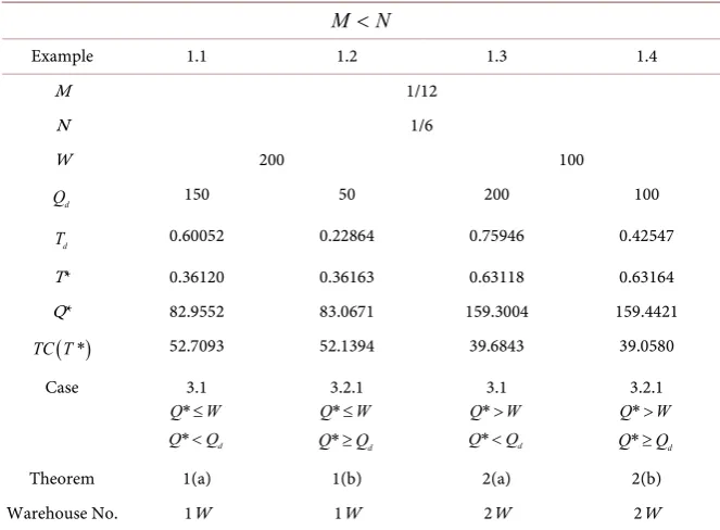
[image:17.595.206.538.190.434.2]

Summarizing the above numerical results, we have the following Table 1 and Table 2.

Table 1. Summary on optimal solutions for Examples 1.1-1.4.

N M<

Example 1.1 1.2 1.3 1.4

M 1/12

N 1/6

W 200 100

d

Q 150 50 200 100

d

T 0.60052 0.22864 0.75946 0.42547 T* 0.36120 0.36163 0.63118 0.63164 Q* 82.9552 83.0671 159.3004 159.4421

( )

*

TC T 52.7093 52.1394 39.6843 39.0580 Case 3.1

*

Q ≤W

* d

Q <Q

3.2.1

*

Q ≤W

* d

Q ≥Q

3.1

*

Q >W

* d

Q <Q

3.2.1

*

Q >W

* d

Q ≥Q

Theorem 1(a) 1(b) 2(a) 2(b)

[image:17.595.199.538.463.737.2]

Warehouse No. 1W 1W 2W 2W

Table 2. Summary on optimal solutions for Examples 2.1-2.4.

M N≥

Example 2.1 2.2 2.3 2.4

M 1/6 3/4

N 1/12

W 200 100 200 100

d

Q 50

d

T 0.22864 0.22864 0.22864 0.22864 T* 0.36117 0.63180 0.36166 0.62982 Q* 82.9473 159.4901 83.0776 158.8857

( )

*

TC T 51.3978 38.3262 44.9099 31.9370 Case 3.2.2

*

Q ≤W

* d

Q ≥Q

*

M T≤ +N

3.2.2

*

Q >W

* d

Q ≥Q

*

M T≤ +N

3.2.3

*

Q ≤W

* d

Q ≥Q

*

M T> +N

3.2.3

*

Q >W

* d

Q ≥Q

*

M T> +N Theorem 1(c) 2(c) 1(d) 2(d)

(18)

From Table 1 and Table 2, some managerial insights can be obtained.

1) As the predetermined order quantity Qd increases, then the retailer’s total relevant cost _{TC T}

( )

* _{increases, the optimal replenishment time}_T*_{and the} optimal order quantity _Q*_{decrease. It reveals that if predetermined order} quantity is large, then it is not beneficial for the retailer.

2) As the capacity of own-warehouse W increases, the optimal replenishment time _T*_{and the optimal order quantity}_Q*_{decrease. It reveals that adopt} one-warehouse is advantageous for the retailer, since need not to rent a ware-house, but the optimal retailer’s total relevant cost is higher.

3) As the upstream trade credit period M increases, the optimal retailer’s total relevant cost _{TC T}

( )

* _{decreases, the optimal replenishment time}_T*_{and the} optimal order quantity _Q*_{increase. It reveals that the longer upstream trade} credit period, the less the retailer’s total relevant cost is.

4) As the downstream trade credit period N increases, then the retailer’s total relevant cost _{TC T}

( )

* _{increases, since the retailer need to pay more interest} than earned. Further, the optimal replenishment time _T*_{and the optimal} or-der quantity _Q*_decrease.

5) As the difference M N− _{increases, then the retailer’s total relevant cost}

( )

*

TC T decreases. It reveals that the longer the upstream trade credit period and the shorter the downstream trade credit period will cause the retailer’s total relevant cost to be less. It will be more profitable for the retailer. Further, the op-timal replenishment time _T*_{and the optimal order quantity}_Q*_{decrease in} the case of Q W> _{, whereas increase in the case of} Q W≤ _.

6. Conclusions

In this paper, an inventory model for deteriorating items with limited storage capacity in a supply chain is developed. The supplier offers a permissible delay in payment linked to order quantity, in the meanwhile, the retailer also provides a downstream trade credit period to its customers. The demand rate is linearly in-creasing with time and the deterioration rate is constant. Simultaneously, the discounted cash flow analysis is also taken into account. The results reveal that 1) as the optimal order quantity is less than the predetermined order quantity ( *

d

Q <Q _{) and the optimal order quantity is not greater than the capacity of}

own-warehouse (_Q*_≤_W_{) will cause more retailer’s total relevant cost than} other cases, since there is no upstream trade credit period allowed, the retailer need to pay more interest than earned.. This is the worst one. 2) As the optimal order quantity is not less than the predetermined order quantity ( *

d Q ≥Q _{), the}

optimal order quantity is greater than the capacity of own-warehouse (_Q*_>_W₎ and N M< _, _{M T}_> *₊_N_{will cause less retailer’s total relevant cost than the} others, since the retailer can earn more interest than paid. It’s more profitable for the retailer in such case. 3) The retailer’s total relevant cost increase as any one of the parameter values W, Qd, N increases, while decreases as M increases.

(19)

period is shorter, and the predetermined order quantity is less, then the retailer’s total relevant cost will be less, it’s more beneficial for the retailer.

The model can be extended in several ways, for example, extend the model to allow for shortages and partial backlogging or partial trade credit. Also, we can add the pricing, quality strategies into consideration.

Conflicts of Interest

The author declares no conflicts of interest regarding the publication of this pa-per.

References

[1] Goyal, S.K. (1985) Economic Order Quantity under Conditions of Permissible De-lay in Payments. Journal of the Operational Research Society, 36, 335-338. https://doi.org/10.1057/jors.1985.56

[2] Shah, N.H. (1993) Probabilistic Time-Scheduling Model for an Exponentially De-caying Inventory When Delay in Payments Is Permissible. International Journal of Production Economics,32, 77-82. https://doi.org/10.1016/0925-5273(93)90009-A [3] Aggarwal, S.P. and Jaggi, C.K. (1995) Ordering Policies of Deteriorating Items

un-der Permissible Delay in Payments. Journal of the Operational Research Society, 46, 658-662. https://doi.org/10.1057/jors.1995.90

[4] Jamal, A.M.M., Sarker, B.R. and Wang, S. (1997) An Ordering Policy for Dete- riorating Items with Allowable Shortages and Permissible Delay in Payments. Jour-nal of the OperatioJour-nal Research Society, 48, 826-833.

https://doi.org/10.1057/palgrave.jors.2600428

[5] Hwang, H. and Shinn, S.W. (1997) Retailer’s Pricing and Lot Sizing Policy for Exponentially Deteriorating Products under the Conditions of Permissible Delay in Payments. Computers & Operations Research,24, 539-547.

https://doi.org/10.1016/S0305-0548(96)00069-X

[6] Chang, H.J. and Dye, C.Y. (2001) An Inventory Model for Deteriorating Items with Partial Backlogging and Permissible Delay in Payments. International Journal of Systems Science, 32, 345-352. https://doi.org/10.1080/002077201300029700

[7] Teng, J.T., Min, J. and Pan, Q.H. (2012) Economic Order Quantity Model with Trade Credit Financing for Non-Decreasing Demand. Omega, 40, 328-335. https://doi.org/10.1016/j.omega.2011.08.001

[8] Teng, J.T. (2002) On the Economic Order Quantity under Conditions of Permissi-ble Delay in Payments. Journal of the Operational Research Society, 53, 915-918. https://doi.org/10.1057/palgrave.jors.2601410

[9] Teng, J.T., Chang, C.T., Chern, M.S. and Chan, Y.L. (2007) Retailer’s Optimal Or-dering Policies with Trade Credit Financing. International Journal of Systems Science,38, 269-278. https://doi.org/10.1080/00207720601158060

[10] Hsieh, T.P., Chang, H.J., Dye, C.Y. and Weng, M.W. (2009) Optimal Lot Size under Trade Credit Financing When Demand and Deterioration Are Fluctuating with Time. International Journal of Information and Management Science, 20, 191-204. [11] Huang, Y.F. (2003) Optimal Retailer’s Ordering Policies in the EOQ Model under

Trade Credit Financing. Journal of the Operational Research Society, 54, 1011-1015. https://doi.org/10.1057/palgrave.jors.2601588