Analytical Algorithm for Systems of Neutral Delay Differential Equations

(1)

https://www.scirp.org/journal/am

ISSN Online: 2152-7393 ISSN Print: 2152-7385

DOI: 10.4236/am.2019.109054 Sep. 25, 2019 753 Applied Mathematics

Analytical

Algorithm

for

Systems

of

Neutral

Delay

Differential

Equations

Aminu

Barde

1,2

,

Normah

Maan

1*

1_{Department of Mathematical Sciences, University Technology Malaysia, Skudai, Malaysia} 2_{Department of Mathematical Sciences, Abubakar Tafawa Balewa University, Bauchi, Nigeria}

Abstract

Delay differential equations (DDEs), as well as neutral delay differential equa-tions (NDDEs), are often used as a fundamental tool to model problems aris-ing from various areas of sciences and engineeraris-ing. However, NDDEs partic-ularly the systems of these equations are special transcendental in nature; it has therefore, become a challenging task or times almost impossible to obtain a convergent approximate analytical solution of such equation. Therefore, this study introduced an analytical method to obtain solution of linear and nonli-near systems of NDDEs. The proposed technique is a combination of Homo-topy analysis method (HAM) and natural transform method, and the He’s polynomial is modified to compute the series of nonlinear terms. The pre-sented technique gives solution in a series form which converges to the exact solution or approximate solution. The convergence analysis and the maxi-mum estimated error of the approach are also given. Some illustrative exam-ples are given, and comparison for the accuracy of the results obtained is made with the existing ones as well as the exact solutions. The results reveal the reliability and efficiency of the method in solving systems of NDDEs and can also be used in various types of linear and nonlinear problems.

Keywords

Homotopy Analysis Method, Natural Transform, He’s Polynomial and Neutral Delay Differential Equations

1. Introduction

Ordinary differential equations (ODEs) are usually used as a fundamental tool in modelling the problems of the real world. However, in most cases, the mathe-matical formulation of real-life problems needs to consider both the present and past states of the system behaviour. Different from (ODEs), DDE is a type of

How to cite this paper: Barde, A. and Maan, N. (2019) Analytical Algorithm for Systems of Neutral Delay Differential Equ-ations. Applied Mathematics, 10, 753-768. https://doi.org/10.4236/am.2019.109054

Received: August 27, 2019 Accepted: September 22, 2019 Published: September 25, 2019

http://creativecommons.org/licenses/by/4.0/

(2)

DOI: 10.4236/am.2019.109054 754 Applied Mathematics differential equation in which the derivative of the unknown function at a cer-tain time is given in terms of the values of the function at previous time [1]. Hence, more reliable models of real problems arising from various field of stu-dies such as; biology, population dynamics, chemistry, and physics, control theory to mention but few are now model using DDEs as well as NDDEs [2] [3]

[4] [5] [6]. Recently series of methods have been developed to find an

approx-imate analytical solution to different types of DDEs [7]-[12]. However, most of these methods have experienced a series of challenges in finding a convergent approximate analytical solution of NDDEs in particular system of such equa-tions. So, scientist and engineers adopt the use of numerical methods as the best approach to approximate the solutions. Therefore, more analytical approaches are highly needed for solving these equations.

This work aims to develop an analytical technique for solving linear and non-linear systems of NDDEs from the combination of HAM and Natural transform. The proposed technique improved on the work of Rebenda and Smarda [12] by introducing the concept of NDDE into Natural transform. In addition, the vari-ous derivatives for both proportional and constants delay of NDDEs were suc-cessfully generated using the Natural transform. This work is also an extension of Efficient Analytical Approach for Nonlinear System of Retarded Delay Diffe-rential equations. This approach was developed by Barde and Maan [13] and solutions to different types of nonlinear systems of retarded DDEs were obtained in a series form which converges to exact or approximate solution.

Thus, based on the results of this pervious works, this research focuses to de-velop a new analytical technique that modifies Efficient Analytical Approach for Nonlinear System of Retarded Delay Differential Equations with aims to obtain approximate analytical solution for both linear and nonlinear system of NDDEs with proportional and constant delays. Using the introduced technique, the He’s polynomial is adjusted in order to ease the computational difficulties of nonli-near terms of such equations. Furthermore, the convergence analysis and the maximum estimated error of the technique are also investigated.

Therefore, in this work we were able to develop a new generating function in Equation (29) that provides a convergent analytical solution to various types of linear and nonlinear system of NDDEs in a series form using few numbers of computational terms and minimal error as compared with the previous niques. Thus, different from some of the existing methods the presented tech-nique provides solution to different form of linear and nonlinear NDDEs with-out any linearization, perturbation or unnecessary assumptions. In Section 4, some illustrative examples are presented in order to show the reliability and effi-ciency of our algorithms over the reference methods.

2. Methods

(3)

DOI: 10.4236/am.2019.109054 755 Applied Mathematics terms of both proportional and constants delays.

HAM is a powerful technique introduced by Lio [14] for solving different types of linear and nonlinear problems. Details on theory and application of HAM can be found in [1] [15] [16] [17] [18].

In recent years natural transform is considered as an active topic in research due to its vast application in solving different type of differential and integral equations [19] [20] [21] [22]. This transform was derived from the renowned Fourier integral which converged to either Laplace or Sumudu transforms de-pending on the values of the transform variables. The basic concepts of natural transform for further use in this research are rendered below.

Definition 2.1 [23]Let t∈ −∞ ∞

(

,

)

, thenthe naturaltransformof the

func-tion v t

( )

isdefinedby:

( )

, e st

( )

d ; ,

(

0,

]

.

v t V s u ∞ v ut t s u

+ −

−∞

= = ∈ ∞

 

 

∫

N (1)

where +

N denotes as natural transform and s u, are transforming variables. Equation (1) can be simplified as [23]

( )

(

]

( )

(

)

( )

(

)

( )

( ) ( )

( )

0

, e d ; , 0,

e d ; , , 0 e d ; , 0,

, ,

st

st st

v t V s u v ut t s u

v ut t s u v ut t s u v t v t

v t H t v t H t V s u V s u

∞

+ −

−∞

∞

− −

−∞

− +

= = ∈ ∞

   

= ∈ −∞ + ∈ ∞

= _ _+ _ _

= _ − _+ _ _

= +

∫

N

N N

(2)

where, H

( )

. is the Heaviside function. Assume the function v t H t

( ) ( )

is

de-fined on +

R and for t∈R then its natural transform can be define over the

set

( )

: , ,1 2 0,

( )

e ,

( )

1

[

0,

)

,

j

t

j

A v t M τ τ v t M τ t j +

 

 

=_ ∃ > < ∈ − × ∞ ∈ _

 

 

Z

as in the given integral:

( )

(

]

0

, e st d ; , 0, .

v t V s u ∞ v ut t s u

+_ _₌ + ₌ − _∈ _∞

 

∫

N (3)

Theorem 2.1 [24] Thegeneralisednaturaltransformofthefunction v t

( )

is

givenas

( )

1 0

!

, .

n n n n

n a u

v t V s u

s ∞

+ +

+ =

= =

 

 

∑

N (4)

Property 2.1 [23] Letabeanon-zeroconstantand v at

( )

∈A then,

( )

1

, .

s v at V u

a a

+_ _₌  

 

  _ _

N (5)

Theorem 2.2 [20]If H_τ istheHeaviside functionandforanyrealnumber 0

(4)

DOI: 10.4236/am.2019.109054 756 Applied Mathematics

( )

1, for

0 for t H t t τ τ τ ≥ 

=  _<



Then the natural transform of the shifted function v t

(

−τ

)

=v t

(

−τ

) ( )

H_τ t

is given by

(

) ( )

e

( )

. s

u

v t H t v t

τ

τ −

+_ ₋ _₌ +_ _

   

N N (6)

Theorem 2.3 [24] Let ( )n

( )

v t be the nth derivatives of the function v t

( )

thenitsnaturaltransformisgivenby

( )

₍ ₎ 1

( )

1 1

, , 0 .

n n n k

n k

n n n k

k

s s

v t V s u V s u v

u u − + + − − + =   = = −  

∑

N (7)

Corollary 2.1 Let ( )n

( )

i

v at be the nth derivatives of the functions v ati

( )

with respect to t,

(

i=1, 2,,N

)

and suppose that N+_v at_i

( )

_=V_i+

(

as u,

)

then we define the following

( )

(

)

( )

(

)

( ) ( )

( )

1 , 1 1

, , 0

n n n k

k n

i n i n i n k i

k

s s

v at V as u V as u v

au au − − + + + − + =   = = −  

∑

N (8)

Proof

Using an induction method, for n=1 and n=2 we respectively obtained the natural transform of first and second derivatives of v ati

( )

that is

( )

(

)

(

)

( )

(

)

(

)

( )

1, 2 2, 2 0 , ,

, 0 0

,

i

i i i

i i

v s

v at V as u V as u

au au

s V as u sv v

v at V as u

au au + + + + + + ′ = = −     ′ − ′′ = = −     N N (9)

Now suppose the result holds for n, then we have to show its also true for 1

n+ . Now from Equation (9) we have

( )

_{( )}

(

( )

_{( )}

)

₍

₎

₍

₎

( )

(

)

( )

( ) ( )

( )

_{( )}

( )

(

)

( )

( ) ( )

( )

1 1, , 1 1 1 1 1 1 1 1 2 1 0 , , 0 , 0 , 0 n

n n i

i i n i n i

n n n n k

k i

i i

n n k

k n k

n n

k

i i

n n k

k

v s

v at v at V as u V as u

au au

v

s s s

V as u v

au _au _au au

s s

V as u v

au au + + + + + + − − + − + = − + + + − + + − + =  ′  _{ =} _ _= = −   _ _     = − −     = −

∑

N N (10)

which is true for n+1 and hence the result. Corollary 2.2

Suppose ( )n

(

)

i

v t−τ are the nth derivatives of the shifted functions v t_i

(

−τ

)

with respect to t, then their natural Transforms can be define as

(

)

( )

( ) ( )

(

)

, 1 1 ₀ 1 e ,

e , lim

s

n u

i n i

s

n n n k

k u

i i

n n k _t

k

v t V s u

s s

V s u v t

(5)

DOI: 10.4236/am.2019.109054 757 Applied Mathematics Proof

Also by induction, for n=1 and n=2 we respectively have the natural transform of first and second derivatives of v ti

(

−τ

)

, that is

(

)

( )

(

)

(

)

( )

(

)

(

)

0 2 0 0 2 1

e , lim

e , lim lim

s u

i i i

t s

u

i i i

t t

i

s

v t V s u v t

u u

s V s u s v t v t v t u u τ τ τ τ τ τ τ − + + → − + + → → ′ − = − −     ′ − − − ′′ − = −     N N (12)

Now assume Equation (11) is true for n and we have to show for n+1. From Equation (12) we have

( )

₍

₎

(

₍

₎

)

( )

₍

₎

(

)

( )

₍ ₎ ( )

₍

₎

( )

₍

₎

( )

₍

₎

1 0 1 0 1 0 1 1 1 1 ( ) 2 ₀ 1

lim

e , lim

n i

n n n t

i i i

n s

n n n k _i

k t

u

i i

n n k t

k

s

n n n k

k u

i i

n n k _t

k

v t s

v t v t v t

u u

v t

s s s

V s u v t

u u u u

s s

V s u v t

u u

τ

τ τ τ

τ τ τ + + + + → − − − + → − + _→ = − + − + − + − + _→ = −  ′  ₋ ₌ _ ₋ _₌  ₋ ₋   _ _   −  _ _ =  − _ − _−     = − _ − _

∑

N N N

(13)

which is true for n+1 and hence the proof.

Another important point to note is that, in both the concept of HAM and natural transform there is no direct approach for the computation of nonlinear terms of the system of NDDEs for both Proportional and constant delays. Therefore, in this research the He’s polynomial will be adjusted for the series calculation of these nonlinear terms.

3. Analysis

of

the

Result

Consider the following n-order system of NDDEs

( )

(

( )

)

( )

_{( )}

( )

(

_{( )}

)

_{[ ]}

,

, , , 0, , 1, , , 1, ,

n

i i

p p

i i j

v t v t

F t v_γ t v_γ t t d i N J M

α

 + 

 

 

= _ _ ∈ =  =  (14)

where

( )

_{( )}

(

( ) ( ) ( )

)

( )

(

)

(

( )

(

_{( )}

)

( )

(

_{( )}

)

( )

(

_{( )}

)

1 2

, 1 , 2 , ,

, , , ,

, , ,

p p p p

N

p k p

p

i j i j i j N i j

v t v v v

v t v t v t v t

γ

γ α α α α

=



for p=0,1, 2,,n−1 and α_{i j}_,

( )

t are the functions of delay terms such that

( )

t max i j,

( )

t

α = _α _

with the given initial conditions

( )

_{( )}

( )

_{( )}

,0

0 , , 0

p p

i i i i

v =v v t =ψ t t< (15)

Now for simplicity we rewrite Equation (14) in the following form

( )

(

)

( ) ( )

( )

i i i i i

L v +v α +R v_γ +F v_γ =g t (16)

(6)

decom-DOI: 10.4236/am.2019.109054 758 Applied Mathematics posed into bounded linear operators Li +Ri (That is there are some positive numbers

α α

i,1, i,2 such that { L vi

( )

γ ≤αi,1 vγ , R vi

( )

γ ≤αi,2 vγ ) with Li as the highest order and Ri as remaining of the linear operators, and Fi are continuous functions satisfy the Lipschitz condition with Lipschitz constants

[ ]

0, i d

µ ∈ ₍ f v_i

( )

− f u_i

( )

≤µ_i v u− ,∀ ∈t

[ ]

0,d }) represent the non-linear

terms.

Take the natural transform of both sides of Equation (16) to obtain:

( )

(

)

( )

i i i i i i i

L v v α R vγ F vγ g t

+_ ₊ _₊ +_ _₊ +_ _₌ +_ _

 

     

N N N N (17)

Note: This research considered two forms of delay functions αi j,

( )

t as fol-lows:

Case I: αi j,

( )

t =a ti j, , where ai j, ∈

( )

0,1 (proportional delay).

Case II: αi j,

( )

t = −t τi j, , where

τ

i j, >0 are real constants (constant delay) Therefore, by substituting the given initial condition into Equation (17), and simplify using the differential properties of natural transform we respectivily obtained the following for the two types of delay as defined in Case I and Case II.

( )

₍ ₎

( )

₍ ₎

( )

( ) ( )

( )

(

)

( ) ( )

( )

1 1 1 1 1 1 0 1 1 1 1 0 0

e 0 lim

0

i

n k n

k i n i n k k i

k

i i

n

i i i n

s n n k

k k

u

i i k i _t i i

k n

i i i n

u

v t v a t v

s

a a

u

R v F v g t s

u

v t v t v v t

s u

R v F v g t s γ γ τ γ γ τ − + − + + − = + − − + − − → = +     + −  +    _ _         + _ + − _=   _ _ + − + −   _ _       + _ + − _=

∑

N N N N (18)

where ai=maxai j,  and τi =maxτi j, 

Now from Equation (18) we can define the following nonlinear operators

( )

₍ ₎

(

)

₍ ₎

( )

(

)

(

( )

)

( )

(

)

( )

(

)

1 1 1 1 1 1 0 1 1 1

; ; ; 1 9

; ;

; ; e ; 0 lim ;

;

i

n k n

k i i i n i i n k k i

k

i i

n

i i i

n

s n n k

k k

u

i i i i k i _t i i

k n

i n

u

N t q t q a t q

s

a a

u

R t q F t q g t s

u

N t q t q t q t q

s u

R t q s

γ γ

τ

γ

φ φ φ φ

φ φ

φ φ φ φ φ τ

φ − + − + + − = + − − + − − → = +     = + − +         _ _         + _ + − _   _ _ = + − + −       _ _ _ _   +

∑

N N N

N _ +F_i

(

φ_γ

( )

t q;

)

−g t_i

( )

_

(19)

where q∈

[ ]

0,1 is an embedding parameter, φ_i

( )

t q; are functions of variables

t and q.

So, by means of HAM we can construct the following Homotopy Equations as

(

1 q

)

φi

( )

t q; vi,0

( )

t h qH t Ni i

( )

i φγ

( )

t q;

+_ _ _ _

− N _ − _= _ _ (20)

where +

N denotes as natural transform, v_i_,0

( )

t are initial approximations of

( )

i

(7)

DOI: 10.4236/am.2019.109054 759 Applied Mathematics Now, from Equation (20) as q=0 and q=1 we respectively obtained the following equation.

( )

,0

, 0 ,1

i i

t v t

t v t

φ

=

= (21)

Thus, as q increases from 0 to 1, the solutions φ_i

( )

t q, vary from the initial approximations vi,0

( )

t to the exact solutions v ti

( )

. In topology, this type of variation is called deformation and Equation (20) is called zero-order deforma-tion equadeforma-tion.

Therefore, the Taylor series expansion of φ_i

( )

t q, with respect to q can be obtained as

( )

,

( )

1

, , 0 m

i i i m m

t q t v t q

φ φ ∞

=

= +

∑

₍₂₂₎

where

( )

0

; 1

!

m i

im m

q t q v t

m q

φ

= ∂

Suppose that the initial approximations vi,0

( )

t , auxiliary parameters hi and the auxiliary function H ti

( )

are properly chosen so that the series in Equation (22) converges at q=1, that is

( )

,0

( )

,

( )

1 ,1

i i i m m

t v t v t

φ ∞

=

= +

∑

₍₂₃₎

Define vectors

( )

, ,0 , ,1 , , ,

i n t = vi t vi t vi n t 

v  (24)

By differentiate Equation (20) m times with respect to q and setting q=0 and finally divided by m! we obtain the so called mth-order deformation equa-tion as

( )

, , 1 i , 1

i m m i m i i y m i m

v t χ v t h H t R t +

− −

 − =  

  v 

N (25)

where

( ) ( )

1

( )

, , 1 1

0

, 1

1 !

i

m i i

y m i m m

q

N t q

R t

m q

φ −

− −

=

∂ _ _

  =

v  ₋ _∂ (26)

and

0, 1

1, 1

m

m m

χ =  ≤_>



By taking the inverse natural transform on both sides of Equation (25) we ob-tained

( )

, , 1 _i , 1

i m m i m i i y m i m

v t =χ v − t +hN−H t R v − t  (27)

Therefore, vi m,

( )

t for m≥1 can be easily obtained from Equation (27), at

(8)

( )

,

( )

0 M i i m

m

v t v t =

=

∑

₍₂₈₎ Hence, as M→ ∞ the following recursive relations of Equations (14) and

(15) for the two type of delay as defined respectively in Case I and Case II are obtained

( ) (

)

( )

(

)

( )

(

)

(

)

( )

( ) (

)

( )

(

)

(

)

( )

1 2

, , 1 , 1

1 1 1

1

, 1 , 1

, , 1 , 1

1 1 0 1 1 1

1 1 0

, , , , 1

1 0 lim

N

i m m i i m i n i m i

i

k n

k

i m n k k i

k i

n

i n i m i m i

i m m i i m i i m i

k n

k

i m k i _t i

k

v t h v t h v a t

a

u

h v

a s

u

h R v t H v v v g t m

s

v t h v t h v t

u

h v v

s

γ γ γ γ

χ χ χ τ χ − − − − − − + = − + − − − − − − − → = = + +   − −  +     _ _ + _ _ + − __ ≥   = + + − − − +

∑

 N N N

N

(

)

( )

(

)

(

₁

)

( )

1

, 1 , 1 , , _N , 1

k i

n

i n i m i m i

t

u

h R v t H v v g t m

s γ γ γ

τ − − + − −  ₋     _ _ + _ _ + − __ ≥    N N (29)

Now, the nonlinear operators F vi

( )

γ are expanded as series of modified He’s polynomials Hi m, −1

(

vγ1,vγ2,,vγn)

)

define as

(

)

, 1 2 ,

0 0 1 , , , ! m m p

i m N m i p

p

q

H v v v F q v

m q

γ γ γ γ

= ₌

 

∂

=  

∂ _

∑

_

 (30)

where vγ,i=

(

vi,1,vi,2,,vi N,

)

and vγ,p =

(

v1,p,v2,p,,vN p,

)

.

The proof for Case II (constant delay) is of the same process with that of Case I. Theorem 3.1 Assume

(

C D

[ ]

, .

)

isaBanachSpaceandlet v_{i m}_,

( )

t be

de-fined in

(

C D

[ ]

, .

)

, where v_{i m}_, are definein formof an operators, that is

( )

(

( )

)

, , 1

i m i i m

v t = A v ₋ t suchthat

( )

_, _, ₁

( )

i

i y m i m

A v = −N−R _v ₋ t _ and

( )

, ,

[ ]

i i i

A v −A u ≤δ u−v ∀v u∈C D (31)

where δi=

(

αi,1+αi,2+µi

)

d for some δi∈

( )

0,1 . Then Ai have unique fixed points in C D

[ ]

. Furthermore, the Homotopy series in Equation (23) converged

uniquelly to the solutions v ti

( )

(their respective fixed points in C D

[ ]

) of Eq-uations (14) and (15).

Proof

Let _C D

( )

, . _ be the Banach space of all continuous functions on C D

( )

,

and from definitions of L Ri, i and Fi in Equation (16) then we have to show that the

{ }

vi m, are Cauchy sequences in C D

( )

, . . Now from Equation (19) we have

( )

₍ ₎

(

)

( )

(

( )

)

, , , , 1 , , 1

1 1 1 , , 1 1 1

2 ; ;

1

1 0 0

i i

i m i p y m i m y p i p

i n i i

i

n k n

k k

i m i p

k n k

k _i

v v R t R t

t q a t q

(9)

( )

(

)

( )

(

)

( )

(

) (

)

{

}

(

)

, 1 , 1

, 1 , 1 , 1 , 1 , 1 , 1

,1 ,2 , 1 , 1 , 1 , 1

; ;

n

i i m i p n

i i m i p i

i i m i p i i m i p i i m i p

i i i i m i p i i m i p

u

R t q t q

s

F t q t q g t

L v v R v v F v v

v v v v

φ φ

α α µ δ

+

− −

− +

− − − − − −

− − − −



+ _ −

 

+ − − 



 

≤ _ − + − + − _

≤ + + − ≤ −

N

N N

(32)

For m= +p 1, we have

2

, 1 , , , 1 , 1 , 2 ,1 ,0

q

i p i p i i p i p i i p i p i i i

v + −v ≤δ v −v − ≤δ v − −v − ≤≤δ v −v (33)

Hence, for all m p, ∈N with m≥ p, by means of Equation (33) and using

triangle inequality we seccessively obtained the following

, , , , 1 , 1 , 2 , 1 ,

1 2

,1 ,0 ,1 ,0 ,1 ,0

1

1 ,0 ,1 ,0

0 0

1 ,0

1 . 1

i m i p i m i m i m i m i p i p

m m p

i i i i i i i i i m n

p k p k

i i i i i i i i

k k

p i i i

i

v v v v v v v v

v v v v v v

v v v v

v v

δ δ δ

δ δ δ δ

δ

− − − +

− −

− − ∞

= =

− ≤ − + − + + −

≤ − + − + + −

= − ≤ −

  = −  ₋   

∑

 

(34)

Since δ <i 1 then for arbitrary εi we can find some large η ∈i N such that

(

)

,1 ,0

1

i i

v v

η ε δ

δ < −

−

Therefore, choosing p m, >N then we obtain the following

(

)

, , ,1 ,0 ,1 ,0

,1 ,0

1

1 1

i i p

i m i p i i i i i i

i i i i

v v v v v v

v v

ε δ

δ ε

δ δ

−

   

− ≤ − _ _< − _ _=

− − −

    (35)

This shows that

{ }

vi m, are Cauchy sequences in C D

[ ]

, and hence the se-quences converged. And the Proof is now completed. The proof for Case II (constant delay) is of the same process with that of Case I.

To establish the proof for the uniqueness of these solutions, let v ti

( )

and

( )

i

u t be two distinct solutions of Equations (14) and (15). According to

Equa-tion (16) we have

( )

1

( )

( ) ( )

i i i i i i

v t +v α =L− _g t −R vγ −F vγ _ (36)

where 1 i

L− are the inverse operators defined by

( )

0 . d

t

∫

. Since v ti

( )

and

( )

i

u t are distinct solutions of Equations (14) and (15), so from Equation (36)

we obtain the following equation

(

)

(

)

(

)

(

)

(

)

(

)

( )

(

)

, ,

0

2,1

d

i i i i

t

i i i i i i i i

t

i i i i i i i

i i i i i i i i

v u v u

v u R v u F v u t

R v u F v F u t

v u v u d v u

α α

α µ δ

− + −

 

≤ − = − _ − + − _

 

≤ _ − + − _

≤ − + − ≤ −

∫

(10)

DOI: 10.4236/am.2019.109054 762 Applied Mathematics According to Equation (37) we have

(

1−δ_i

)

v_i−u_i ≤0 and since δ_i∈

( )

0,1 then v_i −u_i ≤0 implies that vi=ui and hence the proof.

Theorem 3.2 SupposetheHomotopyseriesinEquation (23) convergestothe solutions v ti

( )

of Equations (14) and (15) and let the approximations of

( )

i

v t are givenbythe truncutedseries _,

( )

0 M

i m m= v t

∑

. Then the maximum

ab-soluteerrorisestimatedtobe

( )

,

( )

,0

0 1

n M

i

i i m i

m i

v t v t δ v

δ =

− ≤

−

∑

(38)

Proof

According to Theorem 3.1 and Equation (34) we have

( )

, , ,0

1

n i

i m i p i

i

v v δ v t

δ

− ≤

− As m→ ∞ then v_{i m}_, →v t_i

( )

, so we have

( )

, ,0

( )

1

n i

i i p i

i

v t v δ v t

δ

− ≤

− (39)

Since δi∈

( )

0,1 then 1− ≤δi 1 and from Equation (39) we have

( )

,

( )

,0

( )

0 1

n M

i

i i m i

m i

v t v t δ v t

δ =

− ≤

−

∑

(40)

The Proof is now complete.

4. Examples

and

Discussion

The application of the proposed technique will be presented in this section. This involve solving some problems of linear and nonlinear systems of NDDEs with both proportional and constant delays.

Example 4.1 [10]Firstweseekforasolutionofthefollowing 2-dimensional linearsystemofNDDEswithconstantdelay

( )

(

)

( )

(

)

1 1 2

2 1 1

1 4 , 0 2

1 , 0 2

v t v t v t t

′ = ′ − + ≤ ≤

′ = − − ≤ ≤ (41)

( )

2

( )

(

2( )1 2

)

_[

_]

1 2

1

e , e e , 1, 0 .

2 t

t t

v t = − v t = − − − − t∈ −

Take the natural transform to both sides of Equation (41) and simplify further using Equation (11) to get

( )

(

)

(

)

( )

2

1 1 2

2

2 1 1

1

e 1 e 4 0

1 1

e 1 1 0

2

s

u u

v t v t v t

s s

u

v t v t v t

s s

−

+ +

 

− − − −  =

  _ _ _ _

 

 

− − + − − =

   

  _ _  

N N

(42)

From Equation (42) define a non-linear operator

( )

(

)

(

)

( )

2

1 1 1 2

2

2 2 1 1

1

; ; e ; 1 e 4 ;

1 1

; ; e 1 1; ;

2

s

u u

N t q t q t q t q

s s

u

N t q t q t q t q

s s

φ φ φ φ

−

+ +

 

= − − − −

  _ _  

     

 

 

= − − + − −

     

    _ _  

N N

(11)

DOI: 10.4236/am.2019.109054 763 Applied Mathematics Now using Equation (29) the recursive relation of Example 4.1 can be ob-tained as

( ) (

)

( )

(

)

(

)

(

)

( )

(

)

( ) (

)

( )

(

)

(

)

(

)

( )

2

1, 1 1, 1 1 1 1

1 1 2, 1

2

2, 2 2, 1 2

2 2 1, 1

1

1 1 1 e

1

1 e 1

2

, 1

m m m m

m

m m m m

m

v t h v t h v t h

s u

h R v t

s

v t h v t h

s u

h R v t m

s

χ χ

− −

− +

−

− −

− +

−

 

= + − − − − _ − _

 

 _ _

−  _ _

 

 

= + − − _ − _

 

 _ _

+ _ _ __ ≥

 

N

N N

N

N N

(44)

By choosing an initial approximations of v1,0

( )

t =1 and

( )

(

)

2 2,0

1

e 1

2

v t = −

and using Equation (44) we obtained the following

( )

(

)

( )

(

)

( )

(

)

(

)

( )

(

)(

)

( )

(

)(

)

(

)

( )

(

)

(

)(

)

(

)(

)

2 2

1,1 1 2,1 2

2 2 2

1,2 1 2 1

2 2

2,2 2 1 2 2

2 2 2 2

1,3 1 2 1 2 1

2 2

2 3 2 2 2

2,3 1 2 1 2 1 2

3 2 2

2 2 2

2 e 1 , e 1

2 e 1 2 e 1

2 e 1

3 e 1 2 e 1

2

e 1 2 e 1

3

2 e 1

v t h t v t h t

v t h h t h t

v t h h h h t

v t h h h h t h t

v t h h t h h h h t

h h h t

= − − = −

= − − − −

= + + −

= − − − −

= − − − + −

+ + + −

(45)

Following the same process remaining terms of vi m,

( )

t for m≥3 can be obtained. Putting 1

₍

₂

₎

1

3 e 1

h =

− and h2= −1 in Equation (45), then the fifth order approximation of Example 4.1 is given as

( )

(

) (

)

(

)

(

)

(

)

(

)

2 3 4 5 6

1

2 2 2 2 2 3

2

2 4 2 5 2 6

4 2 4 4

1 2 2

3 3 15 45

1 2

e 1 e 1 e 1 e 1

2 3

1 2 2

e 1 e 1 e 1

3 15 45

v t t t t t t t

v t t t t

t t t

= − + − + − + +

= − − − + − − −

+ − − − + − +



(46)

The series solutions in Equation (46) converged to exact solutions

( )

2

( )

(

2( )1 2

)

1 2

1

e , e e

2 t

t t

v t = − v t = − − − − of Equation (41).

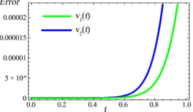
Therefore, the fifth order approximated series of the derived algorithm in Eq-uation (29) was successfully generates the closed form solution of Example 4.1 with minimum error as shown in Figure 1 While in most applications only nu-merical approximations was obtained. For instance, in [10] the numerical ap-proximation of this problem was computed using Implicit Block method with the maximum absolute error of 1.47320 when the tolerance was 1 × 10−10_{in a} to-tal number of 25 steps.

(12)

Figure 1. The behaviour of maximum absolute errors between the exact solution and fifth-order approximation of Example 4.1.

( )

(

)

(

( )

)

( )

(

)

2 3

1 1 1 1

2 2 2 1

2 2 e

3

1

1 , 1

2 2 3

t

v t v t v v t t

t t

v t v v t v t

−

 

′′′ = ′′′ − _{ }+ + +  

   

′′′ = ′′′_{ }+ ′ − _{ } ≥

   

(47)

with initial functions

( )

2

[

]

1 e , 2 , 2, 0

t

t t t t

φ

=

φ

= ∈ −

and the given initial conditions

( )

1 1 1

2 2 2

0 1, 0 1, 0 1

0 0, 0 0, 0 2

v v v

′ ′′

= = =

′ ′′

= = =

Take the natural transform to both sides of Equation (47) and simplify further using Equation (11) to get

( )

(

( )

)

( )

(

)

2 3 2

2 ₃

1 2 3 3 1 1

3

2 2 2 1

1

e 2 e 0

2

8 2 1 0

2 3

t t

u u u t

v t v v t t

s s s s

t u t

v t v t v

s

+ + − −

+ +

     

− + + − + + + =

 _{ } _ _ _{ } _

  _{ }

 

 ₋  ₋  ₋  ₌

   

 _{ }  _{ }

   

N N

(48)

From Equation (48) define a non-linear operator

( )

(

)

( )

(

)

2

1 1 2 3

3 2

2 ₃

1 1

3

2 2 2 2 1

1

; ;

e ; ; 2 e

2

; ; 8 ; 2 1 ; 0

2 3

t t

u u

N t q t q

s s s

u t

q t q t

s

t u t

N t q t q q t q

s

φ φ

φ φ φ φ

+

+ − −

+ +

 

= − + +

   _{ } _

   

 

   

− _ _ _+ + + _

 

 

     

= − − − =

  _ _ __ _ _ __

  _ _ __ _ _ __

N

N N

(49)

Now using Equation (29) the recursive relation of Example 4.2 can be ob-tained as

( ) (

)

(

)

( )

(

)

(

)

( )

( ) (

)

( )

(

)

( )

1

2

1, 1 1, 1 1 2 3

3

1 3 1 1, 1 1, 1 1

3

2, 2 2, 1 2 1 2 3 2 2, 1

1 1

, ,

4

2

N

m m m m

m m

m m m m m

u u

v t h v h

s s s u

h R v t H v v g t

s

t u

v t h v t h v h R v t

s

λ λ

χ χ

χ

− −

− +

− −

− +

− − −

 

= + − − _ + + _

 

 _ _

− _ _ + + __

 

 

  _ _

= + −  _{ }− _  _ 

N

N N

[image:12.595.278.473.75.188.2]

(13)

DOI: 10.4236/am.2019.109054 765 Applied Mathematics By choosing an initial approximations of 1,0

( )

1 2 3

2! 3!

t t

v t = + +t + and

( )

2 2,0

v t =t and using Equation (50) we obtained the following

( )

2 2 2

3 4 5

1,1 1 1 1

2

6 1

3 4 5

2,1 2 2 2

1 e 5 4e 16e 5

6 72 1080

1098e 506

1145

1 1 1

3 27 108

v t h t h t h t

h t v t h t h t h t

− − −

−

 +   +   −  = −_ _ −_ _ −_ _

     

 + 

+  

 

= − − +_

(51)

By putting h1= −1 and h2 = −2 in the series Equation (51) we obtained the approximate solution of Example 4.2 as

( )

2 2 2 2

3 4 5

1

2

6

2 3 4 5

2

1 e 5 4e 16e 5

1

2 6 72 1080

1098e 506

1145

2 2 1

3 27 54

t

v t t t t t

t

v t t t t t

− − −

−

 +   +   −  = + + +_ _ +_ _ +_ _

     

 + 

−  

 

= − + + +_

(52)

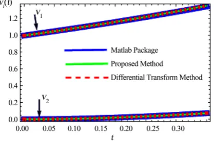
Using only one iteration of the derived algorithm (first order) in Equation (29) a good approximation of Example 4.2 was successfully obtained. Since this problem has no exact solution therefore, Figure 2 shows the comparison be-tween approximate solution obtained by the proposed technique, Matlab Pack-age DDENSD and the result obtained by Rebenda and Smarda [12] using an al-gorithm based on the combination of the method of steps and differential trans-form method (DT).

[image:13.595.270.479.555.693.2]

Threrefore, from Figure 2 we can observed that there is a good correspon-dence between the first order approximate solution of the proposed tecnique with that of Matlab Package DDENSD and DT. Hence, this shows that the pre-sented method provides reliable results and reduces the computation size as compared with the previous techniques.

(14)

5. Conclusion

This paper presents an efficient analytical approach suitable for solving linear and nonlinear systems of NDDEs with proportional and constant delays via HAM and natural transform. The presented algorithm adjusted the He’s poly-nomial in order to ease the computational difficulties of both proportional and constant delays. Another advantage of this research is that a new algorithm is constructed in Equation (25) which reduces the computational work as com-pared to other methods, produces a much faster convergent approximate solu-tion and handles more complicated problems (as in the case of second example) in applications than other analytical methods. Therefore, the presented approach is efficient and reliable in solving different form of linear and nonlinear systems of NDDEs which can be also applied to solve various types of linear and nonli-near problems.

Acknowledgements

The authors like express their gratitude for financial support from Transdiscip-linary Research Grant Scheme (TRGS) under the research programme of Characte-risation of Spatio-temporal Marine Microalgae Ecological Impact Using Mul-ti-Sensor Over Malaysia Waters for the specific sub-project of Mathematical Mod-elling of Harmful Algal Blooms (HABs) in Malaysia Waters (R.J130000.7809.4L854) funded by the Ministry of Education, Malaysia. Authors also like to appreciate the Universiti Teknologi Malaysia for providing all the necessary support and facilities toward the success of this research.

Conflicts

of

Interest

The authors declare no conflicts of interest regarding the publication of this pa-per.

References

[1] Alomari, A.K., Noorani, Mohd Salmi, M.D. and Nazar, R. (2009) Solution of Delay Differential Equation by Means of Homotopy Analysis Method. ActaApplicandae Mathematicae, 108, 395.https://doi.org/10.1007/s10440-008-9318-z

[2] Batzel, J. and Tran, H.T. (2000) Stability of the Human Respiratory Control System I. Analysis of a Two-Dimensional Delay State-Space Model. Journalof Mathemati-calBiology, 41, 45-79.https://doi.org/10.1007/s002850000044

[3] Liu, L.P. and Kalmár-Nagy, T. (2010) High-Dimensional Harmonic Balance Analy-sis for Second-Order Delay-Differential Equations. JournalofVibrationand Con-trol, 16, 1189-1208.https://doi.org/10.1177/1077546309341134

[4] Bellen, A. and Zennaro, M. (2013) Numerical Methods for Delay Differential Equa-tions. Oxford University Press, Oxford.

[5] Rihan, F.A., et al. (2014) A Time Delay Model of Tumour—Immune System Inte-ractions: Global Dynamics, Parameter Estimation, Sensitivity Analysis. Applied MathematicsandComputation, 232, 606-623.

https://doi.org/10.1016/j.amc.2014.01.111

(15)

DOI: 10.4236/am.2019.109054 767 Applied Mathematics Differential Equations: Parameter Estimation, Nonlinearity, Sensitivity. Applied Mathematics, 12, 63-74.https://doi.org/10.18576/amis/120106

[7] Blanco-Cocom, L., Estrella, G.A. and Avila-Vales, E. (2012) Solving Delay Differen-tial Systems with History Functions by the Adomian Decomposition Method. Ap-pliedMathematicsandComputation, 37, 5994-6011.

https://doi.org/10.1016/j.amc.2011.11.082

[8] Bellour, A. and Bousselsal, M. (2014) Numerical Solution of Delay Integro-Differential Equations by Using Taylor Collocation Method. MathematicalMethodsinthe Ap-pliedSciences, 37, 1491-1506.https://doi.org/10.1002/mma.2910

[9] Duarte, J., Januario, C. and Martins, N. (2016) Analytical Solutions of an Economic Model by the Homotopy Analysis Method. Applied Mathematical Sciences, 10, 2483-2490.https://doi.org/10.12988/ams.2016.66188

[10] Ishak, F. and Ramli, M. S.B. (2015) Implicit Block Method for Solving Neutral Delay Differential Equations. AIPConferenceProceedings, 1682, Article ID: 020054.

https://doi.org/10.1063/1.4932463

[11] Rebenda, J., Šmarda, Z. and Khan, Y. (2015) A Taylor Method Approach for Solving of Nonlinear Systems of Functional Differential Equations with Delay.

[12] Rebenda, J. and Šmarda, Z. (2019) Numerical Algorithm for Nonlinear Delayed Differential Systems of nth Order. AdvancesinDifferenceEquations, 2019, Article No. 26.https://doi.org/10.1186/s13662-019-1961-3

[13] Barde, A. and Maan, N. (2019) Efficient Analytical Approach for Nonlinear System of Delay Differential Equations. ComputerScience, 14, 693-712.

[14] Liao, S.J. (1992) The Proposed Homotopy Analysis Technique for the Solution of Nonlinear Problems. Ph.D. Thesis, Shanghai Jiao Tong University, Shanghai. [15] Liao, S.J. (2003) Beyond Perturbation: Introduction to the Homotopy Analysis

Me-thod. Chapman and Hall/CRC, New York. https://doi.org/10.1201/9780203491164 [16] Liao, S.J. and Cheung, F. (2003) Homotopy Analysis of Nonlinear Progressive Waves

in Deep Water. JournalofEngineeringMathematics, 45, 105-116.

[17] Liao, S.J., Su, J. and Chwang, T.A. (2006) Series Solutions for a Nonlinear Model of Combined Convective and Radiative Cooling of a Spherical Body. International JournalofHeatandMassTransfer, 49, 2437-2445.

https://doi.org/10.1016/j.ijheatmasstransfer.2006.01.030

[18] Odibat, Z., Momani, S. and Xu, H. (2010) A Reliable Algorithm of Homotopy Analysis Method for Solving Nonlinear Fractional Differential Equation. Applied MathematicalModelling, 34, 593-600.https://doi.org/10.1016/j.apm.2009.06.025 [19] Khan, Z.H. and Khan, W. (2008) N-Transform-Properties and Applications. NUST

JournalofEngineeringSciences, 1, 127-133.

[20] Belgacem, F.B.M. and Silambarasan, R. (2012) Maxwell’s Equations Solutions by Means of the Natural Transform. International Journalof Mathematics in Engi-neering, ScienceandAerospace, 3, 313-323.https://doi.org/10.1063/1.4765477 [21] Loonker, D. and Banerji, P.K. (2014) Natural Transform and Solution of Integral

Equations for Distribution Spaces. AmericanJournalofMathematicsandSciences, 3, 65-72.

[22] Al-Omari, S.K.Q. (2017) On q-Analogues of the Natural Transform of Certain q-Bessel Functions and Some Application. Filomat, 31, 2587-2598.

https://doi.org/10.2298/FIL1709587A

(16)

DOI: 10.4236/am.2019.109054 768 Applied Mathematics https://doi.org/10.1063/1.4765477