A Lagrange Relaxation Based Approach to Solve a Discrete Continous Bi Level Model

(1)

https://www.scirp.org/journal/ojop ISSN Online: 2325-7091

ISSN Print: 2325-7105

DOI: 10.4236/ojop.2019.83009 Sep. 25, 2019 100 Open Journal of Optimization

A Lagrange Relaxation Based Approach to

Solve a Discrete-Continous Bi-Level Model

Zaida E. Alarcón-Bernal

1

, Ricardo Aceves-García

2

1_{Department of Biomedical Systems Engineering, Universidad Nacional Autónoma de México, Mexico City, Mexico} 2_{Department of Systems Engineering, Universidad Nacional Autónoma de México, Mexico City, Mexico}

Abstract

In this work we propose a solution method based on Lagrange relaxation for discrete-continuous bi-level problems, with binary variables in the leading problem, considering the optimistic approach in bi-level programming. For the application of the method, the two-level problem is reformulated using the Karush-Kuhn-Tucker conditions. The resulting model is linearized taking advantage of the structure of the leading problem. Using a Lagrange relaxa-tion algorithm, it is possible to find a global solurelaxa-tion efficiently. The algo-rithm was tested to show how it performs.

Keywords

Bi-Level Programming, Lagrange Relaxation, Discrete-Continous Linear Bilevel

1. Introduction

The use of optimization techniques has been a fundamental part of solving prob-lems. However, the most common mathematical programming models are often unsuitable for situations involving more than one goal and more than one deci-sion-maker.

In most cases, decisions about a given process are the result of an interaction between the preferences of a group of individuals, so deciding on a single crite-rion seems insufficient, particularly when the decision-making process is applied to complex organizational environments.

Consequently, it is more realistic to seek the achievement of several objectives at the same time. This implies that problems must be solved according to a crite-rion that satisfies all decision-makers as a whole. As a result, contradictory and incommensurable criteria will commonly appear. This situation has led to the How to cite this paper: Alarcón-Bernal,

Z.E. and Aceves-García, R. (2019) A Lagrange Relaxation Based Approach to Solve a Dis-crete-Continous Bi-Level Model. Open Jour-nal of Optimization, 8, 100-111.

https://doi.org/10.4236/ojop.2019.83009

Received: August 22, 2019 Accepted: September 22, 2019 Published: September 25, 2019

(2)

DOI: 10.4236/ojop.2019.83009 101 Open Journal of Optimization

development of multi-objective optimization.

Another way to consider multiple objectives is through bilevel optimization problems, which involve two decision-makers and also consider interdepen-dence between them. These problems are considered as the generalization of the Stackelberg problem [1] for non-cooperative games.

The bilevel programming problem can be formulated as:

( )

min ,

subject to : , 0 1, ,

where for each fixed solves

min ,

subject to : , 0 1, ,

x

k

y

l

F x y

G x y k p

x y

f x y

g x y l q

≤ =



(1)

where _x∈n1 are the higher level variables controlled by the top-level

deci-sion-maker or “leader”, and _y∈n2 are the lower-level variables controlled by

the lower-level decision-maker or “follower”. _{F f}_, _:n1+n2 → are the upper

and lower goal functions respectively. In the decision process, the leader makes a decision that optimizes his objective function. Once the leader has decided, the follower reacts by seeking to optimize his own objective function.

For bi-level programming problem, its fundamental properties and concepts have been studied since the 1970s. A large number of references can be found in

[2]. In general, a bi-level programming problem is difficult to solve: [3] proved that even the simplest case, as the linear bi-level problem, is NP-hard.

Additionally, in many bi-level programming problems, a subset of variables is restricted to taking discrete values. With these characteristics, [4] [5] and [6]

proposed branch and bound algorithms for mixed and binary integers. [7] de-veloped a branch and bound algorithm to solve binary non-linear mixed integer problems. In the work of [8], it is pointed out that the branch and bound me-thods require linear or non-linear convex functions at the lower level of the bi-level problem to be functional.

[9] proposed fundamental properties to find a solution in bi-level linear pro-grams with binary variables. They suggested penalty function methods to solve discrete bi-level problems.

[10] proposed a reformulation and linearization algorithm for the whole bi-level mixed-integer general problem with continuous variables in the follower using the representation of its convex hull. [11] proposed an algorithm to solve the bi-level quadratic problem and the mixed-integer linear based on parametric programming. More recently, [12] used two algorithms using multiparametric programming to solve bi-level integer problems with the integer variables con-trolled by the first level. [13] proposed an algorithm based on the same strategy for bi-level mixed integer problems where the follower solves an integer prob-lem.

(3)

optimal upper bound. [15] proposed an exact algorithm for the linear mixed-integer bi-level problem with some simplifications. [16] considered integer bi-level prob-lems with the leader objective function being linear-fractional and linear the follower; he proposes an iterative algorithm of cut generation to solve the prob-lem.

Using decomposition techniques, [17] proposed an algorithm based on Bend-ers decomposition to solve the linear mixed integer binary problem; with this method, the target values are bounded, and Karush-Kuhn-Tucker (KKT) condi-tions are used to transform the problem into two problems of one level. Based on the last proposal, [18] and [19] proposed the use of Benders decomposition with a continuous subproblem.

Based on the dual decomposition, [20] proposed a method based on Lagran-gian relaxation to obtain an acceptable solution solving a sequence of single level mixed-integer programs. Their heuristic pretends to solve a bi-level problem with binary variables in both levels, considering that the upper-level constraints do not contain any lower-level variable.

In this work, a solution method for discrete-continuous bi-level problems based on Lagrangian relaxation is presented. For our proposal, the reformulation of the bilevel problem to a single level problem with Karush-Kuhn-Tucker con-ditions is applied. This nonlinear problem can be linearized by taking advantages of the structure of the binary variables of the leader problem. Finally, the prob-lem can be solved with a dual decomposition method.

Due to their complexity, bilevel problems are usually solved by heuristic me-thods. Our proposal allows us to find a global optimal through a decomposition technique, taking advantage of some characteristics of the problems involved. The paper is organized as follows: the following section presents the definition and formulation of the discrete-continuous bi-level problem. In Section 2, the solution algorithm is presented. In section 3 the results of the application of the algorithm are shown.

2. Problem Definition and Mathematical Formulation

In this section, we formulate the discrete linear binary problem (DCBLP), where partial cooperation (or optimistic approach) is assumed [21], in which, if the follower has alternative optimal solutions, choose the one that is the best for the leader. The problem can be written as:

{ }

1 1

,

1 1 1

2 2

2 2 2

min

subject to : min

subject to :

0,1 , 0

x y

y

c x d y

A x B y b

c x d y

A x B y b

x y

+

+ ≤

+

+ ≤

∈ ≥

(2)

where 1

1, 1

n

c d ∈ , 2

2, 2

n

c d ∈ , 1

p

b ∈ , 2

q

b ∈ , 1

1

p n

A ∈ × , 2

1

p n

B ∈ × ,

1

2

q n

A ∈× , 2

2

q n

(4)

When the lower-level problem is linear, it can be reformulated by replacing the lower-level problem with its Karush-Kuhn-Tucker (KKT) conditions [2] [22]:

,

min

x y c x1 +d y1 (3)

subject to:

1 1 1

A x+B y≤b (4)

2 2 2

A x+B y≤b (5)

(

)

T

2 2 2 0

b A x B y

λ

− − = ₍₆₎

(

T

)

2 2 0

d +λ B y= (7)

{ }

0,1 , , 0

x∈ y

λ

≥ (8)

where

T T T T

2 2 2 2

d y≥ −

λ

B y≥

λ

A x−

λ

b (9)

For a given selection of the leader problem, the problem can be reformulated by relating the primal and dual constraints and requiring the duality gap to be zero. By including the equation:

T T T

2 2 2

d y=

λ

A x−

λ

b (10)

satisfaction of both complementarity constraints is guaranteed. Then, the problem (2) can be written as:

,

min

x y c x1 +d y1 (11)

subject to:

1 1 1

A x+B y≤b (12)

2 2 2

A x+B y≤b (13)

T 2 2

B d

λ

− ≤ (14)

T T

2 2 2

d y=

λ

A x−

λ

b (15)

{ }

0,1 , , 0

x∈ y

λ

≥ (16)

Considering the problems (11)-(16), the term λx= = µ µ1,,µn₁, where

i

µ is the i-th column of µ, can be linearized [17] [18] [23] and Constraint (15) can be rewritten to obtain the following equivalent problem:

,

min

x y c x1 +d y1 (17)

subject to:

1 1 1

A x+B y≤b (18)

2 2 2

A x+B y≤b (19)

T 2 2

B d

λ

− ≤ (20)

1

T T

2 2 2

1

n i i i

d y µ A λ b

=

(5)

(

1

)

1, , ; 1, , 1

li l M xi l q i n

µ

≥

λ

− − =  =  (22)

1

1, ,

i i n

µ ≤λ = _ ₍₂₃₎

T

1, ,

l Mx l q

µ

≤ =  (24)

0

µ ≥ (25)

{ }

0,1 , , 0

x∈ y

λ

≥ (26)

where M is a large positive number.

With Constraints (22)-(25), it is ensured that variables µli take value zero if

0

i

x = and λl if xi =1, i=1,,n1, l=1,,q.

To avoid the use of binary variables, the problem can be transformed into the following model equivalent to the problem (17)-(26):

,

min

x y c x1 +d y1 (27)

subject to:

1 1 1

A x+B y≤b (28)

2 2 2

A x+B y≤b (29)

T 2 2

B d

λ

− ≤ (30)

1

T T

2 2 2

1

n i i i

d y µ A λ b

=

∑

− ₍₃₁₎

(

1

)

1, , ; 1, , 1

li l M xi l q i n

µ

≥

λ

− − =  =  (32)

1

1, ,

i i n

µ ≤λ =  (33)

T

1, ,

l Mx l q

µ

≤ =  (34)

0

µ ≥ (35)

2

x≤x (36)

0≤ ≤x 1, ,yλ≥0 (37)

Constraint (36) is considered as a complicated constraint so that it can be du-alized. From this idea, the following section proposes a solution method for the DCBLP.

3. Solution Algorithm

Lagrange Relaxation

Considering the problem (27)-(37), Constraint (36) as complicated constraint, and a given

u

≥

0

. A lagrangian relaxation is defined by:

(

)

1

2 1 1

,

1 1 1 2 2 2

T 2 2

T T

2 2 2

1

min

subject to :

x y

n i i i

c x d y u x x

A x B y b

B d

d y A b

λ

µ λ

=

+ + −

+ ≤

− ≤

(6)

(

)

1

1 T

1 1, , ; 1, ,

1, ,

0

0 1, , 0

li l i

i

l

M x l q i n

i n

Mx l q

x y µ λ µ λ µ µ λ ≥ − − = = ≤ = ≤ = ≥ ≤ ≤ ≥   

 (38)

where the dual function

ω

( )

u is defined as the Lagrange subproblem:

( )

(

)

1

2 1 1

,

1 1 1 2 2 2

T 2 2

T T

2 2 2

1

min

subject to :

x y

n i i i

u c x d y u x x

A x B y b

B d

d y A b

ω λ µ λ = = + + − + ≤ + ≤ − ≤ =

∑

−

(

)

1

1 T

1 1, , ; 1, ,

1, ,

0

0 1, , 0

li l i

i

l

M x l q i n

i n

Mx l q

x y µ λ µ λ µ µ λ ≥ − − = = ≤ = ≤ = ≥ ≤ ≤ ≥   

 (39)

From the previous function, for all u≥0

( )

* *

1 1

u c x d y

ω

≤ + ₍₄₀₎

Then, the values of the dual function are lower bounds of the optimal value of (27)-(37). From this definition, we have the duality gap:

( )

* * *

1 1 0

c x +d y −ω u ≥ (41)

To solve the problem, we try to reduce the duality gap, considering that if the problem (27)-(37) is nonconvex, the duality gap is usually greater than zero. How-ever, for convex problems, the duality gap disappears [24].

So the dual problem is to find the vector of multipliers u for which the lower bound given by the dual function is maximum:

( )

max

subject to : 0

u u

u

ω

≥ (42)

If the set of feasible solutions could be available in the feasible region of 39, the problem could be solved by listing all of them as

( )

(

( )

2

)

1 1

,

min s s s s , 1, ,

x y

u c x d y u x x s r

ω = + + − = _ ₍₄₃₎

To solve the problem, a dual decomposition algorithm is proposed, for which a method of dual cutting planes is used. In this method, an approximation of the dual function is maximized and has convergence properties similar to those of the subgradient methods [25].

(7)

( )

(

)

( )

(

)

2 1 1 1 1 1 1

2 1 1

max

subject to :

u

r r r r

u

c x d y u x x

ω

≤ + + −

 (44)

where each constraint is a Lagrange cut.

The optimization of the dual problem consists of the iterative resolution of the master problem whose number of Lagrange cuts increases with each iteration.

With the solution of each master problem, a new value of the multiplier u is obtained, which, when evaluated in the Lagrange subproblem, generates a new cut for the master problem.

When the multiplier generates non-bounded subproblems, a constraint must be entered on the master problem that eliminates the multiplier. This cut is known as a boundary cut and is obtained by solving the boundary subproblem

( )

(

)

1 2 1 1 , 1 1 2 2 T 2 T T

2 2 2

1

min

subject to : 0

0 0 x y n i i i

u c x d y u x x

A x B y

B

d y A b

ω λ µ λ = = + + − + ≤ + ≤ − ≤ =

∑

− 1 1 T

0 1, , ; 1, ,

1, ,

0

0 1, , 0

li l i i

l

Mx l q i n

i n

Mx l q

x y µ λ µ λ µ µ λ − − ≥ = = ≤ = ≤ = ≥ ≤ ≤ ≥   

 (45)

If the optimal solution is a negative value, a boundary cut must be entered in the master problem with the form:

( )

(

2

)

1 1

0≤c xr +d yr+u xr− xr (46)

In this way, the Lagrangian relaxation algorithm iterates between a master problem formed by Lagrange and boundary cuts and a subproblem that eva-luates the proposed multipliers.

Lagrangian Relaxation Algorithm

The structure of the Lagrangian relaxation algorithm considering the above in-terpretation is described below:

Step 0. Initialization k=0, =10−6

Step 1. Solve the Lagrangian Relaxation Master Problem

( )

(

)

( )

(

)

2 1 1 2 1 1 max

subject to : if generate a Lagrange cut

0 if generate a boundary cut

u

k k k k k

u

c x d y u x x u

ω

ω ≤ + + −

≤ + + −

(8)

Get the value of k

u and go to step 2.

Step 2. Solve the boundary subproblem (45). If *

( )

0

u

ω

≥ _{go to step 3. In}

another case, obtain the solution k

x , form the corresponding boundary cut, and

go to step 1.

Step 3. Solve the Lagrange subproblem (39). Get the solution k

x , form the

cor-responding Lagrange cut, and go to step 4.

Step 4. If uk−uk− <1  stop. Otherwise go to step 1.

4. Results and Discussion

4.1. Comparisons

In the literature, some articles consider the same type of problems that in this work. Those problems were used to test the performance of the proposed algorithm.

Numerical experiments were performed on an Intel Core i7 2.5 GHz PC with 8.0 GB RAM, compiling 64-bit GAMS 24.7.3 for Windows with the CPLEX and LINDO solvers. Table 1 shows the results obtained when using the algorithm and its comparison with published works.

Based on the obtained results from the examples, the algorithm reaches the op-timum in a very short time and with little iteration: 2, 4, 3, and 4 respectively.

4.2. Test of Algorithm

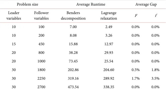
To show the algorithm operation solving an application problem, sixty-one prob-lems were tested, for which the leader and follower solutions are presented. The performance of the algorithm was measured using the execution time and com-paring the obtained solutions with those corresponding to the single-level re-formulation with Karush-Kuhn-Tucker conditions and with the Benders de-composition method proposed in [18]. The results are shown in Table 2.

The experiments were performed on an Intel Core i7 2.5 GHz PC with 8.0 GB RAM, compiling 64-bit GAMS 24.7.3 for Windows with the CPLEX and IPOPT solvers.

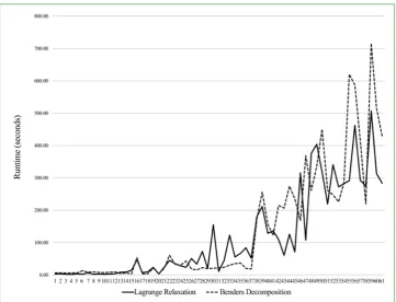
The behavior of the algorithm, in general, is good as can be seen in Figures 1-3. Execution time is reasonable. Even for problems of 30 binary variables con-trolled by the leader problem and 2700 by the follower, the maximum running time was 12 minutes. Using a Lagrange relaxation algorithm, it is possible to find a global solution efficiently.

5. Conclusions

In this paper, we propose an algorithm to solve the discrete-continuous bi-level problem with results very close to the optimum. Lagrangian relaxation is ap-plied to the reformulation to a single-level of the problem considering the Ka-rush-Kuhn-Tucker conditions, and the binary variables are relaxed for the construc-tion of the Lagrange subproblem.

(9)

[image:9.595.176.538.66.215.2] [image:9.595.176.541.248.395.2]

DOI: 10.4236/ojop.2019.83009 108 Open Journal of Optimization Figure 1. Comparison of the optimal value of the leader objective function.

Figure 2. Comparison of the optimal value of the follower objective function.

[image:9.595.177.539.428.704.2]

(10)

[image:10.595.211.540.89.270.2]

DOI: 10.4236/ojop.2019.83009 109 Open Journal of Optimization Table 1. Comparison of results.

No. No. Variables Reference Results in _reference Algorithm _results Running _{time (s)}

Leader Follower

1 4 3 [5] F= −1011.67 F= −1011.67 2.294

4673.34

f= − f = −4673.34

2 2 2 [27] F= −3.25 F= −3.25 3.247

6

f = − f = −6

3 1 1 [4] F=13 F=13 2.169

1

f = f =1

4 1 2 [17] F= −961.69 F= −960 4.94

4673.36

f= − f = −4616

Table 2. Lagrange relaxation algorithm results of test examples.

Problem size Average Runtime Average Gap

Leader

variables Follower variables decomposition Benders relaxation Lagrange F f

10 100 7.00 2.49 0.0% 0.0%

10 200 8.08 3.26 0.0% 0.0%

15 450 15.88 12.97 0.0% 0.0%

20 800 38.28 29.93 0.0% 0.0%

20 1000 73.45 25.54 0.0% 0.0%

30 1800 202.86 204.60 0.5% 1.8%

30 2250 319.16 289.92 1.7% 3.5%

30 2700 473.54 338.35 0.0% 0.0%

in relatively short times, being 12 minutes the maximum time necessary to find a solution, corresponding to a problem with 30 binary variables in the leader prob-lem and 2700 in the follower, two restrictions on the leader and 5610 on the fol-lower.

As a future work, the approach will be used without considering the single-level reformulation of the bilevel problem and the consideration of more than one objective in the leader function.

The method can be used for problems involving cooperative decision-making at two levels, e.g. allocation of resources at minimum cost considering maximi-sation of the level of service, location of unwanted facilities, among others.

Acknowledgements

[image:10.595.210.539.301.481.2]

(11)

Conflicts of Interest

The authors declare no conflicts of interest regarding the publication of this pa-per.

References

[1] Von Stackelberg, H. (1934) Marktform und gleichgewicht. Springer, Berlin. [2] Colson, B., Marcotte, P. and Savard, G. (2007) An Overview of Bilevel

Optimiza-tion. Annals of Operations Research, 153, 235-256.

https://doi.org/10.1007/s10479-007-0176-2

[3] Ben-Ayed, O. and Blair, C.E. (1990) Computational Difficulties of Bilevel Linear Pro-gramming. Operations Research, 38, 556-560.

https://doi.org/10.1287/opre.38.3.556

[4] Moore, J.T. and Bard, J.F. (1990) Mixed Integer Linear Bilevel Programming Prob-lem. Operations Research, 38, 911-921. https://doi.org/10.1287/opre.38.5.911

[5] Wen, U.P. and Yang, Y.H. (1990) Algorithms for Solving the Mixed Integer Two-Level Linear Programming Problem. Computers and Operations Research, 17, 133-142.

https://doi.org/10.1016/0305-0548(90)90037-8

[6] Bard, J.F. and Moore, J.T. (1992) An Algorithm for the Discrete Bilevel Program-ming Problem. Naval Research Logistics, 39, 419-435.

https://doi.org/10.1002/1520-6750(199204)39:3<419::AID-NAV3220390310>3.0.CO;2-C

[7] Edmunds, T.A. and Bard, J.F. (1992) An Algorithm for the Mixed-Integer Nonli-near Bilevel Programming Problem. Annals of Operations Research, 34, 149-162.

https://doi.org/10.1007/BF02098177

[8] Dempe, S. (2003) Annotated Bibliography on Bilevel Programming and Mathemat-ical Programs with Equilibrium Constraints. Optimization, 52, 333-359.

https://doi.org/10.1080/0233193031000149894

[9] Vicente, L., Savard, G. and Judice, J. (1996) Discrete Linear Bilevel Programming Problem. Journal of Optimization Theory and Applications, 89, 597-614.

https://doi.org/10.1007/BF02275351

[10] Ko, C.A. (2005) Global Optimization of Mixed-Integer Bilevel Programming Prob-lems. Computational Management Science, 2, 181-212.

https://doi.org/10.1007/s10287-005-0025-1

[11] Faísca, N.P., Dua, V., Rustem, B., Saraiva, P.M. and Pistikopoulos, E.N. (2007) Pa-rametric Global Optimisation for Bilevel Programming. Journal of Global Optimi-zation, 38, 609-623. https://doi.org/10.1007/s10898-006-9100-6

[12] Domínguez, L.F. and Pistikopoulos, E.N. (2010) Multiparametric Programming Based Algorithms for Pure Integer and Mixed-Integer Bilevel Programming Prob-lems. Computers and Chemical Engineering, 34, 2097-2106.

https://doi.org/10.1016/j.compchemeng.2010.07.032

[13] Köppe, M., Queyranne, M. and Ryan, C.T. (2010) Parametric Integer Programming Algorithm for Bilevel Mixed Integer Programs. Journal of Optimization Theory and Applications, 146, 137-150. https://doi.org/10.1007/s10957-010-9668-3

[14] Mitsos, A. (2010) Global Solution of Nonlinear Mixed-Integer Bilevel Programs.

Journal of Global Optimization, 47, 557-582.

https://doi.org/10.1007/s10898-009-9479-y

(12)

[16] Sharma, V., Dahiya, K. and Verma, V. (2014) A Class of Integer Linear Fractional Bilevel Programming Problems. Optimization, 63, 1565-1581.

https://doi.org/10.1080/02331934.2014.883509

[17] Saharidis, G.K. and Ierapetritou, M.G. (2009) Resolution Method for Mixed Integer Bi-Level Linear Problems Based on Decomposition Technique. Journal of Global Optimization, 44, 29-51. https://doi.org/10.1007/s10898-008-9291-0

[18] Fontaine, P. and Minner, S. (2014) Benders Decomposition for Discrete-Continuous Linear Bilevel Problems with Application to Traffic Network Design. Transporta-tion Research Part B: Methodological, 70, 163-172.

https://doi.org/10.1016/j.trb.2014.09.007

[19] Caramia, M. and Mari, R. (2015) A Decomposition Approach to Solve a Bilevel Ca-pacitated Facility Location Problem with Equity Constraints. Optimization Letters, 10, 997-1019.

[20] Rahmani, A. and MirHassani, S.A. (2015) Lagrangean Relaxation-Based Algorithm for Bi-Level Problems. Optimization Methods and Software, 30, 1-14.

https://doi.org/10.1080/10556788.2014.885519

[21] Dempe, S. (2002) Foundations of Bilevel Programming. Springer Science & Busi-ness Media, Berlin.

[22] Bard, J.F. (1998) Practical Bilevel Optimization: Algorithms and Applications, Vo-lume 30. Springer Science & Business Media, Berlin.

[23] Cao, D. and Chen, M.Y. (2006) Capacitated Plant Selection in a Decentralized Manufacturing Environment: A Bilevel Optimization Approach. European Journal of Operational Research, 169, 97-110. https://doi.org/10.1016/j.ejor.2004.05.016

[24] Bertsekas, D.P. (1999) Nonlinear Programming. Athena Scientific, Belmont. [25] Nowak, I. (2006) Relaxation and Decomposition Methods for Mixed Integer

Nonli-near Programming, Volume 152. Springer Science & Business Media, Berlin. [26] De Haro, S.C.L., Galán, A.R. and Moreno, A.B. (2004) Modelado de algoritmos de

descomposición con gams.