A New Analytical Solution for the Distance Modulus in Flat Cosmology

ISSN Print: 2161-4717

DOI: 10.4236/ijaa.2019.91005 Mar. 14, 2019 51 International Journal of Astronomy and Astrophysics

A New Analytical Solution for the Distance

Modulus in Flat Cosmology

Lorenzo Zaninetti

Physics Department, via P. Giuria 1, Turin, Italy

Abstract

A new analytical solution for the luminosity distance in flat ΛCDM cosmolo-gy is derived in terms of elliptical integrals of first kind with real argument. The consequent derivation of the distance modulus allows evaluating the Hubble constant, H0=69.77 0.33± , Ω =M 0.295 0.008± and the

cosmo-logical constant,

(

)

52 2

1 1.194 0.017 10

m −

Λ = ± × .

Keywords

Galaxy Groups, Clusters, and Superclusters, Large Scale Structure of the Universe, Cosmology

1. Introduction

The release of two catalogs for the distance modulus of Supernova (SN) of type Ia, namely, the Union 2.1 compilation, see [1], and the joint light-curve analysis (JLA), see [2], allows matching the observed distance modulus with the theoret-ical distance modulus of various cosmologies. In this fitting procedure, the cos-mological parameters are derived in a scientific and reproducible way.

We now focus our attention on the flat Friedmann-Lemaître-Robertson-Walker (flat-FLRW) cosmology. A first fitting formula has been derived by [3] and an approximate solution in terms of Padé approximant has been introduced by [4]. The presence of the elliptical integrals of the first kind in the integral for the lu-minosity distance in flat-FLRW cosmology has been noted by [5] [6] [7]. As a practical example the luminosity distance can be expanded into a series of or-thonormal functions and the two cosmological parameters turn out to be

0 70.43 0.33

H = ± _and Ω =_M 0.297 0.002± _{, see [8]. This paper first introduces} in Section 2 a framework useful to build a new solution for the luminosity

dis-How to cite this paper: Zaninetti, L. (2019) A New Analytical Solution for the Distance Modulus in Flat Cosmology. In-ternational Journal of Astronomy and Astrophysics, 9, 51-62.

https://doi.org/10.4236/ijaa.2019.91005 Received: January 11, 2019

Accepted: March 11, 2019 Published: March 14, 2019

Copyright © 2019 by author(s) and Scientific Research Publishing Inc. This work is licensed under the Creative Commons Attribution International License (CC BY 4.0).

http://creativecommons.org/licenses/by/4.0/

DOI: 10.4236/ijaa.2019.91005 52 International Journal of Astronomy and Astrophysics

tance in flat-FLRW cosmology, which will be derived in Section 3.

2. Preliminaries

This section reviews the adopted statistical framework, the ΛCDM cosmology, and an existing solution for the luminosity distance in flat-FLRW cosmology.

2.1

.

The

Adopted Statistics

In the case of the distance modulus, the merit function _χ2 _is

(

) (

)( )

2

2

1 ,

N _i

i th

i i

m M m M z

χ

σ

=

 − − − 

=  

 

 

∑

(1)

where N is the number of SNs,

(

m M−

)

_i is the observed distance modulus evaluated at redshift zi, σi is the error in the observed distance modulus eva-luated at zi, and

(

m M z−

)( )

i th is the theoretical distance modulus evaluated at zi, see formula (15.5.5) in [9]. The reduced merit function χred2 is

2 2 _,

red NF

χ =χ (2) where NF N k= − _{is the number of degrees of freedom, N is the number of} SNs, and k is the number of parameters. Another useful statistical parameter is the associated Q-value, which has to be understood as the maximum probability of obtaining a better fitting, see formula (15.2.12) in [9]:

2

1 GAMMQ , ,

2 2

N k

Q= − _ − χ _

  (3)

where GAMMQ is a subroutine for the incomplete gamma function.

The goodness of the approximation in evaluating a physical variable p is eva-luated by the percentage error δ

100,

approx

p p p

δ = − × ₍₄₎

where papprox is an approximation of p.

2.2

.

The

Standard Cosmology

We follow [10], where the Hubble distance DH is defined as

H 0

.

c D

H

≡ ₍₅₎

The first parameter is ΩM

0

M 2

0

8π _,

3

G H

ρ

Ω = ₍₆₎

where G is the Newtonian gravitational constant and ρ0 is the mass density at

the present time. The second parameter is ΩΛ

2

2 0

, 3

c H

Λ

Λ

DOI: 10.4236/ijaa.2019.91005 53 International Journal of Astronomy and Astrophysics

where Λ is the cosmological constant, see [11]. These two parameters are con-nected with the curvature ΩK by

M Λ K 1.

Ω + Ω + Ω = ₍₈₎ The comoving distance, DC, is

( )

C _{H 0}

d z z D D E z ′ = ′

∫

(9)

where E z

( )

is the “Hubble function”

( )

(

)

3

(

)

2

M 1 K 1 .

E z = Ω +z + Ω +z + ΩΛ (10)

The above integral does not have an analytical solution but a solution in terms of Padé approximant has been found, see [12].

2.3. A First Formula for a Flat-FLRW Universe

The first model starts from Equation (2.1) in [4] for the luminosity distance, dL,

(

)

(

)

(

)

1 1

L 0 M ₄

1

0 _{M M}

d

; , , 1 ,

1

z

c a

d z c H z

H + _{a a}

Ω = +

Ω + − Ω

∫

(11)

where H0 is the Hubble constant expressed in km·s−1·Mpc−1, c is the speed of

light expressed in km·s−1_{, z is the redshift and a is the scale-factor. The indefinite}

integral, Φ

( )

a , is

(

)

(

)

M ₄ M M d , . 1 a a a a

Φ Ω =

Ω + − Ω

∫

(12)

The solution is in terms of F, the Legendre integral or incomplete elliptic integral of the first kind, and is given in [13].

The luminosity distance is

(

)

(

) ( )

L 0 M

0

1

; , , 1 1 ,

1

c

d z c H z

H z

   

Ω = ℜ + Φ − Φ_{ +} _

 

  (13)

where ℜ means the real part. The distance modulus is

(

m M−

)

=25 5log+ 10

(

d z c HL

(

; , 0,ΩM

)

)

. (14)

3. A New Formula for a Flat-FLRW Universe

The second model for the flat cosmology starts from Equation (1) for the lumi-nosity distance in [14]

(

)

(

)

(

)

L 0 M _{0 3}

0 _{M M}

1 1

; , , d .

1 1

z

c z

d z c H t

H _t

+

Ω =

Ω + + − Ω

∫

(15)

The above formula can be obtained from formula (9) for the comoving dis-tance inserting Ω =K 0 and the variable of integration, t, denotes the redshift.

A first change in the parameter ΩM introduces

M 3

M

1

s= − Ω

DOI: 10.4236/ijaa.2019.91005 54 International Journal of Astronomy and Astrophysics

and the luminosity distance becomes

(

)

(

)

(

)

₍

₎

L 0 _{0 3}

0 ₃ 1

3

1 1

; , , 1 d .

1

1 1

1

z

d z c H s c z t

H _t s s − = + + + − + +

∫

(17)

The following change of variable, t s u u

−

= _{, is performed for the luminosity}

distance which becomes

(

)

(

)

(

)

(

)

(

)

3 3 3 ₁

L 0 2 3 3 3

0

1

; , , 1 1 d .

1 1 s z s s u c u

d z c H s z s u

H s + u u s

+

= − + +

+ +

∫

(18)

Up to now we have followed [14] which continues introducing a new function

( )

T x ; conversely we work directly on the resulting integral for the luminosity distance: which is

(

)

(

)

(

)

(

)

L 0

4 3 4 3

0

4

; , ,

1 3

1 3 1

1 3 2 ,1 4 2 3 1 4 2

3 1

3 1

2 ,1 4 2 3 1 4 2 ,

1 3

d z c H s

s s z

c z s

F

sH s s z

s s F s s   _{+ +}  + + _{  } = − × +  _ + + + _    ₊     − +   + +    (19)

where s is given by Equation (16) and F

(

φ,k

)

is Legendre’s incomplete elliptic integral of the first kind,

( )

sin

0 2 2 2

d

, ,

1 1

t

F k

t k t

φ

φ =

− −

∫

(20)

see [15]. The distance modulus is

(

m M−

)

=25 5log+ 10

(

d z c H sL

(

; , 0,

)

)

, (21)

and therefore

(

)

_{( )}

(

) (

3 4 1 2

)

3

0

1 3 1

1 1

25 5 ln ,

ln 10 3

c z F F s

m M sH  _{+ − +}    − = + −  

  (22)

where

(

)

4

1

1 3

2 ,1 4 2 3 1 4 2

3 1

s s z

F F

s s z

 _{+ +} 

 

= +

 + + + 

  (23)

and

(

)

4 2

3 1

2 ,1 4 2 3 1 4 2 ,

1 3 s s F F s s  ₊    = +  + + 

  (24)

with s as defined by Equation (16).

Data Analysis

DOI: 10.4236/ijaa.2019.91005 55 International Journal of Astronomy and Astrophysics

modulus of SNs has become a common practice, see among others [8] [16] [17]. The best fit to the distance modulus of SNs is here obtained by implementing the Levenberg-Marquardt method (subroutine MRQMIN in [9]). This method re-quires the fitting function, in our case Equation (22), as well the first derivative

(

)

0 m M

H

∂ −

∂ , which has a simple expression, and the first derivative

(

)

M m M

∂ − ∂Ω ,

which has a complicated expression. A simplification can be introduced by im-posing a fiducial value for the Hubble constant, namely 1 1

0 70 km s Mpc

H _{= ⋅} − _⋅ − _,

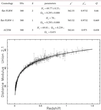
see [2] [18]. We call this model “flat-FLRW-1”, where the “1” stands for there being one parameter. Table 1 presents H0 and ΩM for the Union 2.1

compi-lation of SNs and Figure 1 displays the best fit. The reading of this table allows to evaluate the goodness of the approximation, see (4), in the derivation of the Hubble constant in going from the supposed true value ( 1 1

0 70 km s Mpc

H _{= ⋅} − _⋅ − ₎

to the deduced value ( 1 1

0 69.77 km s Mpc

[image:5.595.210.536.327.682.2]

H _{= ⋅} − _⋅ − _{), which is}

_δ

_{=99.67%. The}

Table 1. Numerical values from the Union 2.1 compilation of _χ2_, 2

red

χ _{and Q, where k}

stands for the number of parameters.

Cosmology SNs k parameters _χ2 2

red

χ Q

flat-FLRW 580 2 H0=69.77 0.33± ; M 0.295 0.008

Ω = ± 562.55 0.9732 0.66

flat-FLRW-1 580 1 H0=70; M 0.295 0.008

Ω = ± 563.52 0.9732 0.669

ΛCDM 580 3 H0=69.81; Ω =M 0.239;

0.651

Λ

Ω = 562.61 0.975 0.658

DOI: 10.4236/ijaa.2019.91005 56 International Journal of Astronomy and Astrophysics

JLA compilation is available at the Strasbourg Astronomical Data Centre (CDS), and consists of 740 type I-a SNs for which we have the heliocentric redshift, z, the apparent magnitude mB in the B band, the error in mB , σ_mB, the parameter X1,

the error in X1, σX1, the parameter C, the error in C, σC, and log10

(

Mstellar

)

. The observed distance modulus is defined by Equation (4) in [2]:

1 b B.

m M− = −Cβ+X α−M +m ₍₂₅₎

The adopted parameters are α=0.141_,

β

=3.101 _and

10

10

19.05 if 10

19.12 if 10stellar

b

stellar

M M

M

M M

− <



= _{− ≥}



 

(26)

see line 1 in Table 10 of [2]. The uncertainty in the observed distance modulus, m M

σ _{− , is found by implementing the error propagation equation (often called} the law of errors of Gauss) when the covariant terms are neglected, see Equation (3.14) in [19],

2 2 2 2 2

1 _B.

m M X C _m

σ − = α σ +β σ +σ  (27)

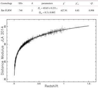
The parameters as derived from the JLA compilation are presented in Table 2

[image:6.595.212.537.394.684.2]

and the fit is presented in Figure 2.

Table 2. Numerical values from the JLA compilation of _χ2_, 2

red

χ and Q, where k stands for the number of parameters.

Cosmology SNs k parameters _χ2 2

red

χ Q

flat-FLRW 740 2 H0=69.65 0.231± ; M 0.3 0.003

Ω = ± 627.91 0.85 0.998

DOI: 10.4236/ijaa.2019.91005 57 International Journal of Astronomy and Astrophysics

As an example the luminosity distance for the Union 2.1 compilation with data as in the first line of Table 1 is

( )

(

)

L 8147.04 1.0

3.1188 1.33542

0.637664 2.63214 ,0.965925 1.75322 Mpc

4.64846

d z z

z F z = +   +     × −_ _ _+ _ +     (28)

when 0< <z 1.5

and the distance modulus is

(

)

25.0 2.17147ln 8147.04 1.0

3.1188 1.3354

0.63766 2.6321 ,0.96592 1.7532 .

4.6484

m M z

z F z  − = + _ +     +  _ × −_ _ _+ _ +     (29)

when 0< <z 1.5

We now derive some approximate results without Legendre integral for the flat-FLRW case and Union 2.1 compilation with data as in Table 1, first line. A Taylor expansion of order 6 around z = 0 of the luminosity distance as given by Equation (19) for the flat-FLRW case and Union 2.1 compilation gives

( )

2 3

L

4 5

0.000423646 4296.57 3344.13 1186.94

979.403 42078.6 Mpc

d z z z z

z z

= + + −

+ − (30)

when 0< <z 0.197.

The upper limit in redshift, 0.197, is the value for which the percentage error, see Equation (4), is δ =1.16%_{. The asymptotic expansion of the luminosity}

distance with respect to the variable z to order 5 for the flat-FLRW case and Un-ion 2.1 compilatUn-ion gives

( )

( )

1 L ₁ 3 2 1 1

14283.5 15802 14283.5 7901.01

1975.25 Mpc

d z z z

z z − − − − + − +  (31)

when 1.27< <z 1.5.

At the lower limit of z=1.27 the percentage error is δ =0.54%. The two above approximations at low and high redshift have a limited range of existence but does not contain the Legendre integral as solutions (28) and (29) which cov-er the ovcov-erall range 0< <z 1.5_.

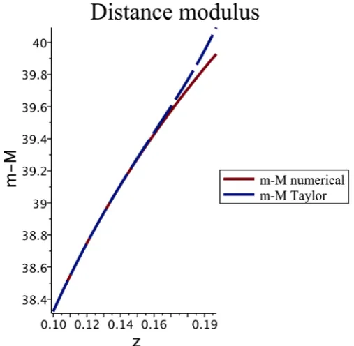
A Taylor expansion of order 6 of the distance modulus as given by Equation (22) around z=0.1 for the flat-FLRW case and Union 2.1 compilation gives

(

)

(

)

(

)

(

)

(

)

2 3

4 5

36.0051 23.1777 109.604 0.1 724.464 0.1

5429.06 0.1 43429.8 0.1

m M z z z

z z

− = + − − + −

− − + − (32)

when 0.1< <z 0.197.

The upper limit in redshift, 0.197, is the value at which the percentage error is

0.14%

[image:8.595.246.500.69.317.2]

DOI: 10.4236/ijaa.2019.91005 58 International Journal of Astronomy and Astrophysics Figure 3. Distance modulus in flat-FLRW cosmology as represented by Equation (22) with parameters as in first line of Table 1 (full red line) and Taylor solution (dash-dot-dash line) (blue line).

The asymptotic expansion of the distance modulus with respect to the variable

z to order 5 for the flat-FLRW case and Union 2.1 compilation gives

(

)

( )

( )

( )

( )

1 1

3 2 5 2

1 2 1

7 2

3 1 4

45.7741 2.17147ln 2.40231 0.842625

0.221081 0.570086 0.150471

0.357849 0.491842 0.179989

m M z z z

z z z

z z z

− −

− − −

− − −

− + − +

+ − −

+ + +



(33)

when 1.27< <z 1.5.

The lower limit in redshift, 1.27, is the value at which the percentage error is

0.54%

δ = . The ranges of existence in z for the analytical approximations here derived have the percentage error <2%, see Equation (4).

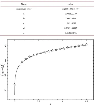
We now introduce the best minimax rational approximation, see [20] [21] [15], of degree (2, 1), for the distance modulus m2,1

( )

z ,

( )

2

2,1 a bz cz .

m z

d ez

+ + =

+ (34) In the case in which the distance modulus is represented by Equation (29) and given the interval

[

0.001,1.5

]

, the coefficients of the best minimax rational approximation are presented in Table 3; the maximum error for the fit is

5

2.2 10−

≈ × _{. Figure 4 displays the data and the fit.}

4. Conclusions

[image:9.595.208.538.112.482.2]

DOI: 10.4236/ijaa.2019.91005 59 International Journal of Astronomy and Astrophysics Table 3. Maximum error and coefficients of the distance modulus for the best minimax rational approximation for the flat-FLRW case and Union 2.1 compilation. Interval of ex-istence

[

0.001,1.5

]

.

Name value

maximum error 2.28881836 × 10−5

a 0.981622279

b 19.6473351

c 1.08210218

d 0.0309164915

e 0.462291896

Figure 4. Distance modulus in flat-FLRW cosmology as represented by Equation (22) with parameters as in first line of Table 1 (full line) and minimax rational approximation (empty stars); Union 2.1 compilation.

of SNs of type Ia allows finding the parameters H0 and ΩM for the two

com-pilations in flat-FLRW cosmology

(

)

1 1

0 69.77 0.33 km s Mpc , M 0.295 0.008

H _{= ± ⋅} − _⋅ − _{Ω = ± (35)}

flat-FLRW-Union 2.1,

(

)

1 1

0 69.65 0.23 km s Mpc , M 0.3 0.003

H _{= ± ⋅} − _⋅ − _{Ω = ± (36)}

flat-FLRW-JLA,

A first comparison with [8] in the case of the Union 2.1 compilation gives a percentage error p=0.93% _{for the derivation of} H₀ and p=0.67% _{for the}

derivation of ΩM. A second comparison can be done with Equation (13) in [22]

(

)

1 1

0 67.27 0.60 km s Mpc , M 0.3166 0.0084

H _{= ± ⋅} − _⋅ − _{Ω = ± (37)}

[image:10.595.206.540.57.309.2]

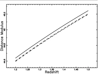
DOI: 10.4236/ijaa.2019.91005 60 International Journal of Astronomy and Astrophysics Figure 5. Distance modulus for ΛCDM cosmology (full line), flat-FLRW-1 (dot-dash-dot- dash line) and flat-FLRW cosmology (dashed line). Parameters as in Table 1 and interval of existence

[

1.2,1.5

]

.

In the case of the Union 2.1 compilation, the percentage error p=3.71% _for the derivation of H0 and p=6.82% for ΩM. A Taylor expansion at low

redshift and an asymptotic expansion are presented both for the luminosity dis-tance and the disdis-tance modulus. A simple version of the disdis-tance modulus is de-termined through the best minimax rational approximation. Adopting the cos-mological parameters found here, the coscos-mological constant Λ _{turns out to be,}

for the Union 2.1 compilation,

(

)

52

2

1 1.19457 0.017 10

m −

Λ = ± × ₍₃₈₎

flat-FLRW Union 2.1, or introducing c=1 _{and the Planck time,} t_p,

(

)

122

2

1 3.12046 0.0462942 10

p

t

−

Λ = ± × (39)

flat-FLRW Union 2.1.

The statistical parameters of the fits are given in Table 1 and Table 2 where the other two models are presented. The values of the _χ2 _{in the above table say}

DOI: 10.4236/ijaa.2019.91005 61 International Journal of Astronomy and Astrophysics

Conflicts of Interest

The author declares no conflicts of interest regarding the publication of this pa-per.

References

[1] Suzuki, N., Rubin, D., Lidman, C., Aldering, G., Amanullah, R., Barbary, K. and Barrientos, L.F. (2012) The Hubble Space Telescope Cluster Supernova Survey. V. Improving the Dark-Energy Constraints above Z Greater than 1 and Building an Early-Type-Hosted Supernova Sample. ApJ,746, 85.

https://doi.org/10.1088/0004-637X/746/1/85

[2] Betoule, M., Kessler, R., Guy, J. and Mosher, J. (2014) Improved Cosmological Con-straints from a Joint Analysis of the SDSS-II and SNLS Supernova Samples. A&A, 568, A22.

[3] Pen, U.L. (1999) Analytical Fit to the Luminosity Distance for Flat Cosmologies with a Cosmological Constant. ApJS, 120, 49. https://doi.org/10.1086/313167 [4] Adachi, M. and Kasai, M. (2012) An Analytical Approximation of the Luminosity

Distance in Flat Cosmologies with a Cosmological Constant. Progress of Theoretical Physics, 127, 145. https://doi.org/10.1143/PTP.127.145

[5] Eisenstein, D.J. (1997) An Analytic Expression for the Growth Function in a Flat Universe with a Cosmological Constant. arXiv:astro-ph/9709054

[6] Liu, D.Z., Ma, C., Zhang, T.J. and Yang, Z. (2011) Numerical Strategies of Compu-ting the Luminosity Distance. MNRAS, 412, 2685.

https://doi.org/10.1111/j.1365-2966.2010.18101.x

[7] Mészáros, A. and Řpa, J. (2013) A Curious Relation between the Flat Cosmological Model and the Elliptic Integral of the First Kind. A&A, 556, A13

https://doi.org/10.1051/0004-6361/201322088

[8] Benitez-Herrera, S., Ishida, E.E.O., Maturi, M., Hillebrandt, W., Bartelmann, M. and Röpke, F. (2013) Cosmological Parameter Estimation from SN Ia Data: A Mod-el-Independent Approach. MNRAS, 436, 854.

https://doi.org/10.1093/mnras/stt1620

[9] Press, W.H., Teukolsky, S.A., Vetterling, W.T. and Flannery, B.P. (1992) Numerical Recipes in FORTRAN. The Art of Scientific Computing. Cambridge University Press, Cambridge.

[10] Hogg, D.W. (1999) Distance Measures in Cosmology. arXiv:astro-ph/9905116 [11] Peebles, P.J.E. (1993) Principles of Physical Cosmology. Princeton University Press,

Princeton, NJ.

[12] Zaninetti, L. (2016) Pade Approximant and Minimax Rational Approximation in Standard Cosmology. Galaxies, 4, 4.https://doi.org/10.3390/galaxies4010004 [13] Zaninetti, L. (2016) An Analytical Solution in the Complex Plane for the

Luminosi-ty Distance in Flat Cosmology. Journal of High Energy Physics, Gravitation and Cosmology, 2, 581. https://doi.org/10.4236/jhepgc.2016.24050

[14] Baes, M., Camps, P. and Van De Putte, D. (2017) Analytical Expressions and Nu-merical Evaluation of the Luminosity Distance in a Flat Cosmology. MNRAS, 468, 927.

[15] Olver, F.W.J., Lozier, D.W., Boisvert, R.F. and Clark, C.W. (2010) NIST Handbook of Mathematical Functions. Cambridge University Press, Cambridge.

DOI: 10.4236/ijaa.2019.91005 62 International Journal of Astronomy and Astrophysics [17] Jones, D.O., Scolnic, D.M., Riess, A.G., Rest, A., Kirshner, R.P., Berger, E., Kessler, R., Pan, Y.C., Foley, R.J., Chornock, R., Ortega, C.A., Challis, P.J., Burgett, W.S., Chambers, K.C., Draper, P.W., Flewelling, H., Huber, M.E., Kaiser, N., Kudritzki, R.P., Metcalfe, N., Tonry, J., Wainscoat, R.J., Waters, C., Gall, E.E.E., Kotak, R., McCrum, M., Smartt, S.J. and Smith, K.W. (2018) Measuring Dark Energy Proper-ties with Photometrically Classified Pan-STARRS Supernovae. II. Cosmological Pa-rameters. The Astrophysical Journal, 857, 51.

[18] Ben-Dayan, I., Gasperini, M., Marozzi, G., Nugier, F. and Veneziano, G. (2013) Av-erage and Dispersion of the Luminosity-Redshift Relation in the Concordance Model. Journal of Cosmology and Astroparticle Physics, 6, 2.

[19] Bevington, P.R. and Robinson, D.K. (2003) Data Reduction and Error Analysis for the Physical Sciences. McGraw-Hill, New York.

[20] Remez, E. (1934) Sur la détermination des polynômes d’approximation de degré donnée. Communications of Kharkov Mathematical Society, 10, 41.

[21] Remez, E. (1957) General Computation Methods of Chebyshev Approximation. The Problems with Linear Real Parameters. Publishing House of the Academy of Science of the Ukrainian SSR, Kiev.