X ray/UV/optical variability of NGC 4593 with Swift : reprocessing of X rays by an extended reprocessor

Advance Access publication 2018 August 2

X-ray/UV/optical variability of NGC 4593 with

Swift

: reprocessing of

X-rays by an extended reprocessor

I. M. M

Hardy,

S. D. Connolly,

K. Horne,

E. M. Cackett,

J. Gelbord,

B. M. Peterson,

M. Pahari,

N. Gehrels,

M. Goad,

P. Lira,

P. Arevalo,

R. D. Baldi,

N. Brandt,

E. Breedt,

H. Chand,

G. Dewangan,

C. Done,

M. Elvis,

D. Emmanoulopoulos,

M. M. Fausnaugh,

S. Kaspi,

C. S. Kochanek,

K. Korista,

I. E. Papadakis,

A. R. Rao,

P. Uttley,

M. Vestergaard

and

M. J. Ward

Affiliations are listed at the end of the paper

Accepted 2018 July 23. Received 2018 July 18; in original form 2017 December 12

A B S T R A C T

We report the results of intensive X-ray, UV, and optical monitoring of the Seyfert 1 galaxy NGC 4593 with Swift. There is no intrinsic flux-related spectral change in any variable component with small apparent variations being due to contamination by a constant hard (reflection) component in the X-rays and the red host galaxy in the UV/optical. Relative to the shortest wavelength band,UVW2, the lags of the other UV/optical bands mostly agree with the predictions of reprocessing of high energy emission by an accretion disc. TheU-band lag is, however, larger than expected, probably because of reprocessed Balmer continuum emission from the distant broad line region (BLR). TheUVW2 band is well correlated with the X-rays but lags by∼6×more than expected if theUVW2 results only from reprocessing of X-rays by the disc. However, if the light curves are filtered to remove variations on time-scales>5 d, the lag approaches the expectation from disc reprocessing.MEMECHOanalysis shows that direct X-rays can be the driver of most of the UV/optical variations if the response functions have tails up to 10 d, from BLR reprocessing, together with strong peaks at short lag (<1 d) from disc reprocessing. For the 5 AGN monitored so far, the observedUVW2 toV-band lags are <

∼2 of disc reprocessing expectations and vary little between AGN. However, the X-ray to UVW2 lags greatly exceed disc reprocessing expectations and differ between AGN. The two most absorbed AGN have the largest excesses, so absorption and scattering may affect these lags, but there is no simple relationship between excess and absorption.

Key words: galaxies: active – galaxies: individual: NGC 4593 – galaxies: Seyfert – ultraviolet: galaxies – X-rays: galaxies.

1 I N T R O D U C T I O N

The origin of the UV and optical variability in AGN, and its rela-tionship to the X-ray variability, are questions of major relevance to understanding the central structures of AGN. One possible ex-planation of UV/optical variability is that variations in the thermal emission from the accretion disc are caused by fluctuations in the inward accretion flow (Ar´evalo & Uttley2006). A second possibil-ity is that X-ray emission from the central corona or very hard UV emission from the very inner edge of the accretion disc illuminates

_{E-mail:[email protected]}

the outer disc, heating it up and causing it to re-radiate (Haardt & Maraschi1991).

The time lag between the high energy emission and the re-radiated lower energy UV/optical emission gives us the distance between these two emission regions. Therefore, by measuring the lags be-tween the high energy emission and a number of UV/optical bands we can map out the temperature structure of the disc. This technique is known as ‘reverberation mapping’ (RM; Blandford & McKee

1982) and has been used to map regions too small to be resolved by direct imaging, e.g. AGN broad line regions (BLR; Peterson2014). The model of a smooth, optically thick, geometrically thin, ef-ficiently radiating accretion disc was first derived by Shakura & Sunyaev (1973, SS) and has been our basic disc model for over

40 yr. In this model, the release of gravitational potential energy from accreting material leads to a temperature profile (in physi-cal units) ofT(R)∝R−3/4_(Mm)˙ 1/4_{. Incident high energy emission} will enhance the existing thermal emission (slightly altering the disc temperature profile). We thus expect a wavelength (λ) dependent lag,τ, between the incident high energy, and re-radiated UV/optical emission, ofτ=R/c∝(M2_m˙

E)1/3λβ whereβ=4/3 and ˙mEis the accretion rate in Eddington units (Cackett, Horne & Winkler

2007). We also expect the optical variations to be smoother and have lower amplitude of variability than the UV variations as they will come from a larger emission region. Both Cackett et al. (2007) and Sergeev et al. (2006) find lags consistent withβ=4/3 between various optical bands. However neither study included X-ray data. A number of observers have studied the relationship between the X-ray and UV or optical wavebands, mostly combining ground-based optical observations with space-ground-based X-ray observations fromRXTE(e.g. Uttley et al.2003; Suganuma et al.2006; Ar´evalo et al.2008,2009; Breedt et al.2010; Lira et al.2011; Cameron et al.

2012). These observations have mostly shown strong X-ray/optical correlations on short time-scales (weeks–months), with the optical lagging the X-rays by∼1 d, but have sometimes shown long-term trends (months–years) in the optical which are not mirrored in the X-rays (e.g. Breedt et al.2009). There are occasional examples where the UV/optical appears to lead the X-rays on short time-scales, in particular in NGC 7469 (Nandra et al.1998) where although the dips in the 30 dRXTEX-ray andIUE1315 Å UV light curve line up with approximately zero lag, the best-defined peak in the UV light curve is 4d before an X-ray peak. There is almost certainly more than one cause of the UV/optical variability with long time-scale variations probably being dominated by accretion rate fluctuations propagating inwards through the disc. Interpretation of the origin of the short time-scale variations depends very much on whether the X-rays lead or lag the UV/optical emission. Although, overall, the observations from the sample of AGN monitored byRXTE

strongly support the conclusion that the optical lags the X-rays, in no individual case is the uncertainty on the lag small enough to be absolutely sure that the optical does lag.

Recent monitoring campaigns withSwift(e.g. Mc_{Hardy et al.} 2014; Shappee et al.2014; Edelson et al.2015; Fausnaugh et al.

2016; Troyer et al.2016; Edelson et al. 2017) have greatly im-proved the measurement of lags between the X-ray, UV, and optical bands and have therefore significantly improved our understanding of the origin of UV/optical variability in AGN. However, these ob-servations have also highlighted questions about the structures of accretion discs, of the importance of the BLR in producing repro-cessed UV and optical emission and about whether X-rays from the central corona or maybe hard UV emission from the inner edge of the accretion disc are driving the longer wavelength UV/optical variability. The above campaigns all show that the longer wave-lengthSwiftUVOT bands lag behind the shortest wavelengthSwift

UV band (UVW2; 193 nm) in a manner which is in agreement with the short time-scale (weeks/months) UV/optical variability of AGN being produced by reprocessing of radiation of shorter wavelength thanUVW2 and coming from a compact region near the black hole. However, Mc_{Hardy et al. (2014) noted that if all of the reprocessing} is being carried out by a surrounding accretion disc, that the disc is either hotter than or larger than we should expect, assuming the SS model and given the mass and accretion rate of the target AGN. All subsequent papers (e.g. Fausnaugh et al.2016) found a similar result. These observations were consistent with microlensing ob-servations (e.g. Dai et al.2010; Morgan et al.2010; Mosquera et al.

2013) which had already pointed out a similar disc size discrepancy.

It was also clear (e.g. Edelson et al.2015; Fausnaugh et al.2016) that the lag in theuband was longer than that in surrounding bands, indicating that the BLR was also contributing to the lags.

There has additionally been the concern that the optical light curves do not look as expected if they arise from reprocessing of X-ray emission from a small central corona, e.g. of size simi-lar to that which we measure from microlensing observations, i.e.

<

∼10RG (Dai et al.2010; Mosquera et al. 2013), or from X-ray low/high energy reverberation, i.e.∼4Rg(Cackett et al.2014;

Em-manoulopoulos et al.2014). The observed optical light curves are smoother than expected and an insufficient fraction of the X-ray emission hits the disc to power the optical variability (e.g. Berkley, Kazanas & Ozik2000; Ar´evalo et al.2008). Larger coronal sizes are required. Gaskell (2008) also notes the energetics problem and pro-poses variations originating independently in different parts of the disc. However, although such a model is useful for explaining the uncorrelated variations between bands which are sometimes seen, it cannot explain the well correlated multiwavelength variations seen in theSwiftobservations. Gardner & Done (2017) proposed an alter-native model in which the X-ray emission does not directly impact on the outer disc but mainly heats up the very inner edge of the disc, which then inflates and re-radiates at hard UV wavelengths on to the outer disc. In this model there should be an additional lag between the X-ray andUVW2 emission, over and above that expected from an extrapolation of the longer wavelength lags down to the X-ray waveband. This additional lag would correspond to the thermal time-scale for the incident X-ray heating to pass through the inner disc to the re-radiation surface. Gardner & Done (2017) note the existence of such a lag when the unfiltered X-ray andUVW2

observations of NGC 5548 are compared. However, Mc_{Hardy et al.} (2014) do not see any additional lag in NGC 5548 if those light curves are filtered to remove variations on time-scales longer than 20 d. In NGC 4151, Edelson et al. (2017) see a very large excess lag between the X-ray andUVW2bands. Unlike in NGC 5548, the excess lag in NGC 4151 is strongly energy dependent, with the highest energy X-rays having the largest lag. NGC 4151 is the most absorbed of the few AGN whose lags have been well studied so far and so the energy dependence may be a function of scattering in the absorbing medium.

So far the number of AGN with accurately measured lags is small. With Swift, lags have been measured well in NGC 5548 (Mc_{Hardy et al.2014; Edelson et al.2015; Fausnaugh et al.2016)} and NGC 4151 (Edelson et al.2017) and less thoroughly in NGC 2617 (Shappee et al.2014) and NGC 6814 (Troyer et al.2016). With

XMM–Newtonlags have been measured in NGC 4395 between the X-ray and one UV (UVW1) and one optical (g) band (Mc_Hardy et al.2016). NGC 4593 has a black hole mass which is almost an order of magnitude lower than that of the other AGN for which multiband monitoring has been performed bySwift. Thus, in 20 d ofSwiftobservations we can probe relative size scales (measured in gravitational radii) which would require monitoring, although at reduced frequency, over a few months for the other AGN. We also note that the AGN in which lags have been measured well so far have been of relatively low accretion rate (NGC 4395 ˙mE∼0.0012, NGC 4151 ˙mE∼0.021, NGC 5548 ˙mE∼0.048). We therefore proposed forSwiftmonitoring of the somewhat higher accretion rate NGC 4593 ( ˙mE∼0.081), allowing us to investigate the importance of accretion rate and disc temperature in determining disc and BLR structure.

In Section 2, we present theSwiftobservations and light curves. The X-ray spectrum is relevant to understanding of lags and disc structure as, in the model of Gardner & Done (2017), the tail of a

luminous hard UV emission component may be expected to show up in at low X-ray energies. Thus, in Section 3, we discuss the time averageSwiftX-ray spectrum and X-ray spectral variability. In Section 4, we discuss the relationships, and lags, between the X-ray and the various UV/optical bands. In Section 5, we compare the lags and the observedUVW2 light curve with the predictions from re-processing of X-rays by a simple SS accretion disc. In Section 6, we present a more sophisticated maximum entropy modelling of the X-ray/UV/optical light curves to derive reprocessing functions which are more complex than that expected from a simple accretion disc and which indicate the importance of reprocessing from the BLR. This topic is addressed in detail in a paper by Cackett et al. (2018) based on parallelHubble Space Telescope(HST) observations of NGC 4593. In Section 7, we compare the present lag measurements of NGC 4593 with those of other AGN and note broadly similar (scaled) lags between the UV and optical bands but differences in the X-ray/UV lags. We draw some brief conclusions regarding the inner structure of AGN.

Just before submission of this paper, the Swift data from this programme were published by another group (Pal & Naik2018). Although there are some similarities, their analysis and conclusions differ from ours in a number of respects, as we shall note below.

2 SWIFTO B S E RVAT I O N S

Swiftobserved NGC 4593 almost every orbit (96 min) for 6.4 d from 2016 July 13 to 18 and thereafter every second orbit for a further 16.2 d. Each observation totalled approximately 1 ks although observa-tions were often split into two, or sometimes more, visits. TheSwift

X-ray observations are made by the X-ray Telescope (XRT; Bur-rows et al.2005) and UV and optical observations are made by the UV and Optical Telescope (UVOT; Roming et al.2005). In total 194 visits satisfying standard good time criteria, such as rejecting data when the source was located on known bad pixels (e.g. seehttps:

//swift.gsfc.nasa.gov/analysis/xrt swguide v1 2.pdf), were made.

The XRT observations were carried out in photon-counting (PC) mode and the UVOT observations were carried out in image mode. X-ray light curves in a variety of energy bands were produced using our own Southampton pipeline which is based upon the standard

Swiftanalysis tasks as described in Cameron et al. (2012). We made flux measurements for each visit thus providing the best available time resolution. In addition, for comparison, a broad-band ‘snap-shot’ X-ray light curve (i.e. one flux point per visit) was produced using the Leicester Swift Analysis system (Evans et al.2007), which was almost identical to our own snapshot light curve. X-ray data are corrected for the effects of vignetting and aperture losses and data with large flux error (>0.15 count s−1_{) are rejected.}

During each X-ray observation, measurements were made in all six UVOT filters, using the 0x30ed mode which provides expo-sure ratios, for theUVW2,UVM2,UVW1,U,B, andVbands, of 4:3:2:1:1:1. UVOT light curves with the same time resolution were made using the Southampton system and also, independently, using a system developed by Gelbord & Edelson (2017). The latter sys-tem includes a detailed comparison of UVOT ‘drop out’ regions, as first discussed in observations of NGC 5548 (Edelson et al.2015). When the target source is located in such regions theUVW2 count rate is typically 10–15per cent lower than in other parts of the de-tector. The drop in count rate is energy dependent, being greatest in theUVW2 band and least in theVband. The new drop-out box regions are based on intensiveSwiftobservations of three AGN, i.e. NGC 5548 (Edelson et al.2015), NGC 4151 (Edelson et al.2017), and the present observations of NGC 4593. Observations falling

in drop-out regions were rejected. We also searched for observa-tions where the fluxes in the six UVOT bands showed a particularly red spectral slope. Such observations almost always fell within a drop-out region and were also rejected.

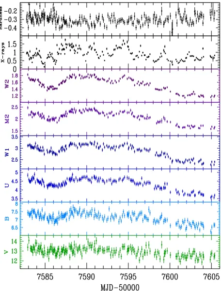
The resultant light curves are shown in Fig.1. We see a close correspondence between all UVOT bands and a reasonable corre-spondence between the X-ray and UVOT bands. In Fig.1we also show the X-ray hardness. The correspondences between these light curves are discussed in the following sections.

3 X - R AY S P E C T R U M A N D VA R I A B I L I T Y

3.1 Time averaged X-ray spectrum

The X-ray spectrum can provide information which is relevant to understanding the inner geometries of AGN and so we have fitted models withXSPECto theSwiftXRT time averaged spectrum derived from the observations shown in Fig.1. The 2–8 keV spectrum is fitted well by a simple power law, with line-of-sight Galactic column cold hydrogen absorber of 1.89×1020_cm−2_{, together with a broad} Gaussian line at 6.4 and a narrow line at∼7 keV. The photon index of the power law is=1.68±0.02. When this model is extended down to 0.3 keV a large negative residual is seen centred on∼1 keV which is consistent with the presence of warm absorbers as detected by previous observers using data fromXMM–Newton(Brenneman et al. 2007) and combined data fromXMM–Newtonand NuStar (Ursini et al. 2016b). Following these studies we add two warm absorbers which results in a good fit to the 0.3–8 keV spectrum with=1.74±0.01. This fit is similar to that of Brenneman et al (=1.75+₋0.02_0.03) except that, unlike them, we do not require an additional ‘soft-excess’ component at low energies.

NGC 4593 is detected in theSwiftBAT 70 month survey (Baum-gartner et al.2013). The spectrum is described as a power law with =1.84+₋0.070.08and flux ( 14–195 keV) of 8.8±0.05×10−11erg

cm−2_s−1_{(https://swift.gsfc.nasa.gov/results/bs70mon/SWIFT J12}

39.6-0519). During the monitoring reported here the average 0.3–

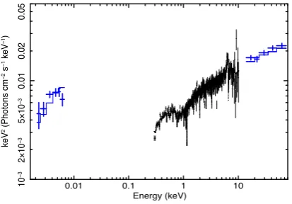
10 keV flux was ∼4.5×10−11 _{erg cm}−2 _s−1_{. To extrapolate a} power law to the BAT energy band, and obtain the observed BAT flux requires=1.73, indicating that the long-term average X-ray luminosity of NGC 4593 has not changed noticeably. Including the BAT data into our spectral fit without any change of normalization, and assuming a simple power law without any high energy cut-off, steepens the overall fit slightly (=1.82+₋0.04_0.05). The overall best fit is shown in Fig.2and the fit parameters are given in Table1.

To the best-fitting model we added, separately, a bremsstrahlung (zbremss) and a Comptonization (comptt) component as used by Brenneman et al. (2007) to describe a soft excess which they find in theirXMM–Newtondata. In ourSwiftdata the normalizations of both components are consistent with zero and the 1σ upper limit on the 0.3–10 keV fluxes for these two components are 6×10−16 and 3.4×10−17_{erg cm}−2_s−1_{, respectively (compared to 2×10}−14 and 6.46×10−14 _{erg cm}−2_s−1_{, respectively, from Brenneman et} al.). We note that Brenneman et al. find variation in the soft excess between different observations so it is possible that we observed withSwiftwhen the soft excess was particularly faint. Pal & Naik (2018) present a 0.3–7 keVSwiftXRT spectrum. It is of much lower S/N than that presented here, possibly being only from a single 1 ks observation. They are therefore able only to fit to a power law, whose slope is not well constrained, and a blackbody. They do not include the warm absorbers or the iron lines.

Figure 1. XRT and UVOT light curves of NGC 4593. The top panel is the hardness ratio defined asH−S/H+SwhereHis the 2–10 keV count rate andSis the 0.5–2 keV count rate. The second from top panel is the 0.5–10 keV count rate for each visit. The lower panels are theUVW2 through toV-band fluxes in units of mJy.

10−3

0.01

5×10−4

2×10−3

5×10−3

EF

E

keV (Photons cm

−2 s −1 keV −1)

0 1 1

−2 0 2

(data−model)/error

Energy (keV)

Figure 2. Best fit, with residuals, to the time averaged XRT and BAT spectrum. The fit parameters are given in Table1.

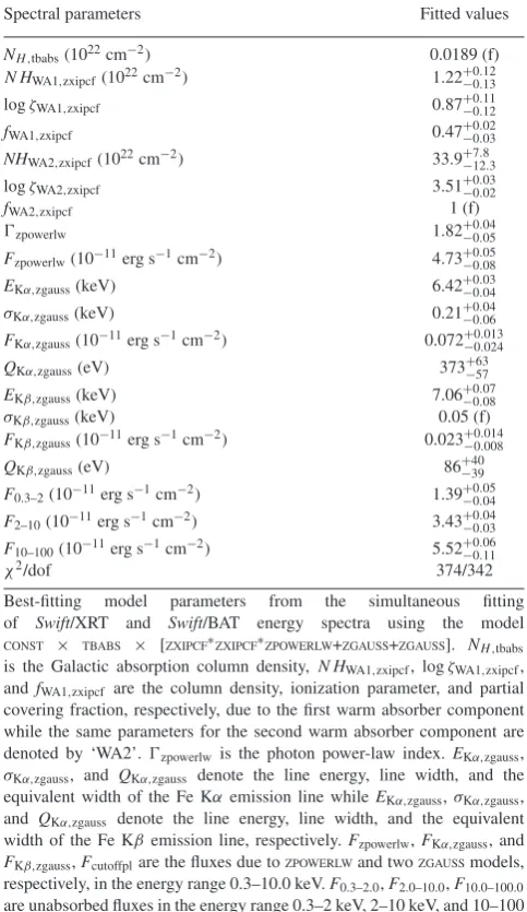
Table 1. X-ray spectral fit parameters.

Spectral parameters Fitted values

NH ,tbabs(1022cm−2) 0.0189 (f) N HWA1,zxipcf(1022cm−2) 1.22+₋00..1213 logζWA1,zxipcf 0.87+₋00..1112

fWA1,zxipcf 0.47+₋00..0203

NHWA2,zxipcf(1022cm−2) 33.9+₋712.8.3 logζWA2,zxipcf 3.51+₋00..0302

fWA2,zxipcf 1 (f)

zpowerlw 1.82+₋00..0405

Fzpowerlw(10−11erg s−1cm−2) 4.73+₋00..0508

EKα,zgauss(keV) 6.42+₋00..0304 σKα,zgauss(keV) 0.21+₋00..0406

FKα,zgauss(10−11erg s−1cm−2) 0.072+₋00..013024

QKα,zgauss(eV) 373+₋6357

EKβ,zgauss(keV) 7.06+₋00..0708 σKβ,zgauss(keV) 0.05 (f)

FKβ,zgauss(10−11erg s−1cm−2) 0.023+₋00..014008

QKβ,zgauss(eV) 86+₋4039

F0.3–2(10−11erg s−1cm−2) 1.39+₋00..0504

F2–10(10−11erg s−1cm−2) 3.43+₋00..0403

F10–100(10−11erg s−1cm−2) 5.52+₋00..0611

χ2/dof 374/342

Best-fitting model parameters from the simultaneous fitting of Swift/XRT and Swift/BAT energy spectra using the model CONST × TBABS × [ZXIPCF∗ZXIPCF∗ZPOWERLW+ZGAUSS+ZGAUSS]. NH ,tbabs is the Galactic absorption column density,N HWA1,zxipcf, logζWA1,zxipcf, andfWA1,zxipcf are the column density, ionization parameter, and partial covering fraction, respectively, due to the first warm absorber component while the same parameters for the second warm absorber component are denoted by ‘WA2’.zpowerlw is the photon power-law index.EKα,zgauss,

σKα,zgauss, and QKα,zgauss denote the line energy, line width, and the equivalent width of the Fe Kαemission line whileEKα,zgauss,σKα,zgauss,

and QKα,zgauss denote the line energy, line width, and the equivalent width of the Fe Kβemission line, respectively.Fzpowerlw,FKα,zgauss, and

FKβ,zgauss,Fcutoffplare the fluxes due toZPOWERLWand twoZGAUSSmodels, respectively, in the energy range 0.3–10.0 keV.F0.3–2.0,F2.0–10.0,F10.0–100.0 are unabsorbed fluxes in the energy range 0.3–2 keV, 2–10 keV, and 10–100 keV, respectively.

0.5 1 1.5 2

−0.6

−0.4

−0.2

0

Hardness (H−S/H+S)

0.5−10 keV counts/s

Figure 3. The X-ray hardness as a function of the 0.5–10 keV count rate. The hardness is defined as (H−S)/(H+S), whereS=0.5–2 keV andH=

2–10 keV count rate.

3.2 X-ray spectral variability and X-ray energy dependence of lags

InSwiftobservations of NGC 4151, Edelson et al. (2017) found large differences in the lag measured between different X-ray bands and theUVW2 band. Although Mc_{Hardy et al. (2014) did not find any} significant differences between the 0.5–2 keV versusUVW2 lags and the 2–10 keV versusUVW2 lags in NGC 5548, the possibility exists that different X-ray bands may come from different locations and so give rise to different lags.

We have therefore made light curves in a variety of narrow and broad X-ray energy bands and have searched for lags between them using a variety of techniques. We can find no measureable lags. For example, usingJAVELIN(Zu, Kochanek & Peterson2011; Zu et al. 2013), we find that the 0.5–2keV band lags the 2–10 keV band by −0.001+₋0.0030.004d. Similarly the lag of the 2–10 keV band by the 0.3–1 keV band is−0.002+0.004

0.005 d.

As an additional method of searching for differences between X-ray bands we have calculated the hardness ratio. The hardness ratio is defined as (H−S)/(H+S), where here the hard (H) band is 2–10 keV and the soft (S) band is 0.5–2 keV. We plot this ratio as a function of time in the top panel of Fig.1. There is little variation. In Fig.3, we plot the hardness ratio against broad-band ( 0.5–10 keV) count rate. Above 0.5 counts s−1_{there is a very slight softening of} the spectrum with increasing count rate. This spectral softening is similar to that found in NGC 4593 by Ursini et al. (2016a) and for AGN in general by Sobolewska & Papadakis (2009). Although they use 0.3–1.5 and 1.5–10 keV as their soft and hard band, respectively, and define hardness ratio asH/Srather than the (H−S)/(H+S) used here, similar results are shown by Pal & Naik (2018).

We note here that below 0.5 counts s−1_{( 0.5–10 keV) data are} limited so it is not clear whether the suggestion of softening with decreasing count rate, at the lowest count rates, is real or not. A softening with decreasing count rate at the lowest count rates has been seen in NGC 1365 (Connolly, Mc_{Hardy & Dwelly2014) and} attributed to unabsorbed (i.e. steep spectrum) X-rays scattered from an accretion disc wind which are still visible even when the direct X-ray emission is heavily absorbed.

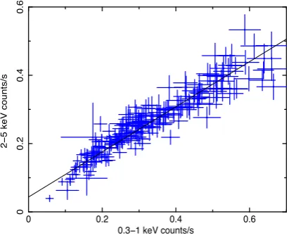
To determine whether the slight softening with increasing lumi-nosity represents a real change in the underlying spectrum we plot, in Fig.4, the 0.3–1 keV count rate against the 2–5 keV count rate. Similar flux–flux plots have been used elsewhere to investigate the

0 0.2 0.4 0.6

00

.2

0

.4

0

.6

2−5 keV counts/s

0.3−1 keV counts/s

Figure 4. The 0.3–1 keV count rate plotted against the 2–5 keV count rate.

reasons behind flux-related X-ray spectral variations (e.g. Taylor, Uttley & Mc_{Hardy2003). Above a 0.3–1 keV count rate of∼0.15} counts s−1_{, there is a strong linear relationship between the count} rates in the two bands with an extrapolation to zero 0.3–1 keV count rate giving a small residual count rate in the harder band. The data are again insufficient to determine whether there is any real deviation from this relationship at the very lowest count rates.

Five combinedXMM–Newtonand NuStar observations have been fitted with a multicomponent model including a power law and a high energy cut-off. From this modelling it is stated that the photon index varies by∼0.25 over a factor 3 in luminosity (Ursini et al.

2016b). The NuStar observations extend to a higher energy than

theSwiftXRT observations but, within the XRT observations, the strong linear relationship between the hard and soft X-ray count rates shows that there is no change of spectral shape of the varying component as a function of luminosity over the large majority of the flux range observed. The weak softening of the overall spectrum with increasing luminosity shown in Fig.3is most simply explained as the combination of a small constant component of hard spectrum together with a varying soft spectrum component. The hard com-ponent may be a reflection comcom-ponent from the disc or BLR. We therefore conclude that, unlike in NGC 4151, all of the XRT energy band varies simultaneously and so, to increase S/N, we hereafter use the 0.5–10 keV band unless stated otherwise.

4 X - R AY / U V- O P T I C A L C O R R E L AT I O N S

4.1 X-ray/UVW2 discrete correlation function

Visual inspection of the X-ray andUVW2 light curves indicates that most of the X-ray flux variations on∼day time-scales have counterparts, though of lesser fractional variability (Table2), in the

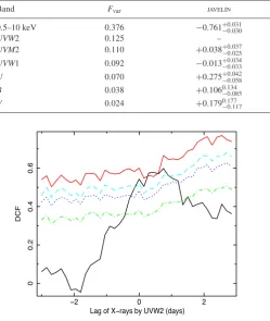
UVW2 light curve. As a basic method of quantifying the relationship between these two bands we show, in Fig.5, the discrete correlation function (DCF; Edelson & Krolik1988) between these two bands together with simulation-based confidence contours. We see that a correlation exists between these two bands at greater than 99 per cent confidence. This degree of confidence between the observed X-ray andUVW2 light curves, without any filtering to remove long-term trends which often distort DCFs, is higher than in all other previous intensive Swift AGN monitoring programs (e.g. Mc_{Hardy et al.} 2014; Edelson et al.2015,2017). The peak lag corresponds to the

UVW2 lagging the X-rays by about half a day. The exact value of the lag will be considered in more detail later.

The confidence contours are calculated in broadly the same way as in our previous papers on X-ray/optical correlations (e.g. Breedt et al.2009). X-ray light curves are simulated with the same vari-ability properties, e.g. power spectral density (PSD) and count rate probability density function (PDF), as for the observed X-ray light curve. The Nper cent confidence levels are defined such that if correlations are performed between the observedUVW2 data and randomly simulated X-ray light curves, only (100−N) per cent of the correlations would exceed those levels. The confidence levels are appropriate to a single trial, i.e. a search at zero lag, approxi-mately what we are searching for here. For a search over a wide lag range where the expected lag was unknown, the confidence levels would be reduced by an amount depending on the ratio of the lag range being searched to the width of the expected corre-lation function (i.e. (ACF W idt h2

X+ACF W idt h2O)1/2, where ACF W idt hXandACF W idt hOare the half-widths of the X-ray and optical autocorrelation functions). If this ratio wasR, then the single-trial confidence level of (100−N) per cent would reduce to (100−RN) per cent. We note that the previous light-curve simula-tion method depended only on the parameters of the X-ray PSD, using the method of Timmer & Koenig (1995). The present light-curve simulation method follows Emmanoulopoulos, Mc_{Hardy &} Papadakis (2013), with code available from Connolly (2015), which also takes account of the count rate PDF. Unlike the method of Timmer & Koenig (1995) which can only produce Gaussianly dis-tributed light curves, this method can produce light curves with any PDF, including the highly non-linear light curves seen in the gamma-ray and TeV bands.

The level and detailed shape of the confidence contours do change, though only very slightly, depending on the model chosen for the X-ray PSD. Here, we used the standard bending power-law model of Mc_{Hardy et al. (2004) with Poisson noise and fixed the} low frequency PSD slope at−1. The PSD derived here from the

SwiftXRT observations is still not very well constrained but a high frequency slope of−1.8 was measured, similar to that (−2.2) found by Summons (2007) fromRXTEandXMM–Newtonobservations. However, even quite large changes in the X-ray PSD model do not change the confidence contours greatly. In almost all tests the peak of the DCF reached a significance level of between∼95 and 99 per cent.

DCFs for the relationship between theUVW2 band and the other UVOT bands all show a strong peak near zero lag with very high significance (>99.9 per cent confidence) and are not shown here. The DCF does not provide a particularly accurate measurement of the value of the lag and so the lag measurements are derived using other methods, below.

4.2 X-ray/UV/optical interband lags

All lags are measured relative to the UVW2 band as theUVW2 band provides the highest significance detections of any of the UVOT bands. Lags, with errors, were measured both usingJAVELIN (Zu et al. 2011, 2013), as previously demonstrated by Shappee et al. (2014), Pancoast, Brewer & Treu (2014), and Mc_{Hardy et al.} (2014) and using the ‘flux randomization/random subset selection’ (FR/RSS) method (Peterson et al.1998) with the interpolation cross-correlation function (ICCF; Gaskell & Sparke1986; Gaskell & Pe-terson1987). The median lag values produced byJAVELINare usually close to the values produced by the FR/RSS method but, as noted by Fausnaugh et al. (2016), the uncertainties are usually smaller,

Table 2. Fvarand lags (d) relative toUVW2 from various correlation methods.

Band Fvar JAVELIN FR/RSS peak FR/RSS centroid

0.5–10 keV 0.376 −0.761₋+₀0._.031₀₃₀ −0.412±0.186 −0.662±0.145

UVW2 0.125 – – –

UVM2 0.110 +0.038+₋0_0..037₀₂₅ +0.057±0.083 +0.069±0.086

UVW1 0.092 −0.013₋+0₀._.034₀₃₃ −0.013±0.078 +0.094±0.109

U 0.070 +0.275₋+0₀._.042₀₅₈ +0.186±0.214 +0.317±0.127

B 0.038 +0.1060.134

−0.085 +0.101±0.208 +0.191±0.175

V 0.024 +0.179₋0.177_0.117 +0.220±0.502 +0.247±0.386

−2 0 2

00

.2

0

.4

0

.6

DCF

Lag of X−rays by UVW2 (days)

Figure 5. Solid black line–discrete cross-correlation function between the X-ray and UVW2 light curves shown in Fig.1. The 68 per cent (dot– dashed, green), 90 per cent (dotted, blue), 95 per cent (dashed turquoise), and 99 per cent (solid red) confidence levels are also shown.

here by a factor∼3 (see Table2). Detailed discussion of these dif-ferences is beyond the scope of this paper but will be included in a futureSwiftsurvey paper (Edelson et al., in preparation). There are other cross-correlations methods, e.g. the maximum interpola-tion interval CCF (MCCF) method (Oknyanskii1993; Oknyansky et al.2017) and the z-transformed DCF (ZDCF) method (Alexander

2013), which again usually produce similar results (e.g. Mc_Hardy et al.2014).

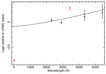
The FR/RSS method produces two alternative lag measurements, based either on the distribution of the values of the centroids of the individual ICCFs (usually measured at 80 per cent of the peak value), or on the distribution of the peak lag values. With asymmet-ric ICCFs, these distribution will differ and provide us with different information. Where an ICCF arises from the sum of a number of contributing lags, the centroid provides us with an estimate of the av-erage lag. The peak highlights the dominant contributor to the lags. In Fig.7, we show the lags measured, from the centroids of the FR/RSS lag distributions. We do not show the lags derived from the peaks of the FR/RSS distributions but we give the values in Table

2. In Fig.8, we show the lags measured usingJAVELINwhich are more like the FR/RSS peak than centroid lags. The lag distributions between theUVW2 and short wavelength bands (X-ray,UVM2) are symmetrical, but tails to longer lags appear in theband vbands (Fig.6) indicating a possible secondary source of lags.

Relative toUVW2, the other UV and optical band lags are very small. With all measurement methods we see that theu-band lag significantly exceeds any interpolation between the lags in bands on

either side. As in NGC 5548 (Edelson et al.2015; Fausnaugh et al.

2016), this excess lag is probably due to a contribution from the BLR as predicted by Korista & Goad (2001) and is discussed in detail for NGC 4593 by Cackett et al. (2018). The lag measured byJAVELINto theUVW1 band is actually negative, though is also consistent with a small positive value. Possibly there is some contribution from [C III] from the BLR to the emission inUVW2 but not inUVW1.

Pal & Naik (2018), although finding lags which increase with wavelength, do not obtain the same lag values as those given here. The main difference between our analyses is that Pal and Naik use 1.5–10 keV as their reference band against which to measure lags in all other bands, from soft X-ray toVband, whereas we measure all other UVOT band lags relative toUVW2. As we see in Fig.1, and as seen in all previousSwiftAGN monitoring campaigns, theUVW2 light curve has the highest S/N of any of the UVOT bands. Also the main change in the character of the variability is between the X-rays andUVW2 whereas the other UVOT bands are quite similar in character toUVW2. Thus, the peak correlation strength between the X-rays andUVW2 is∼0.6 (as shown also by Pal and Naik) whereas the peak correlation strength betweenUVW2 and the other UVOT bands is greater than 0.9. Thus, lag measurements between

UVW2 and the other UVOT bands have much smaller errors than lag measurements between the hard X-ray band and the UVOT bands. We also find no evidence for lags between hard and soft X-ray bands and so we measure a lag betweenUVW2 and the broad 0.5–10 keV X-ray band, which has higher S/N than just the 1.5–10 keV band. Thus, we believe that the lags presented here are a more accurate measurement of the true lags than those presented by Pal and Naik. In Figs7and8, we also plot model lags on the assumption that the variable UV/optical emission is produced by reprocessing of X-ray emission by an accretion disc. To calculate these model lags we broadly follow Kazanas & Nayakshin (2001), Cackett et al. (2007), and Ar´evalo et al. (2008). We first assume that the steady-state temperature structure and emission from the disc, in the absence of X-ray illumination, is as given by Shakura & Sunyaev (1973). We then calculate the new temperature structure following X-ray illumination and hence derive the change in emission, in eachSwift

UVOT band, from every part of the disc. Taking account of the different light traveltimes from each part of the disc to the observer we add up the changes in emission as a function of time to produce the response functions, Fig.9. As previously (e.g. Mc_{Hardy et al.} 2014), we take, as the model lag, the time for half of the reprocessed light to be received. We refer to this lag as the median lag.

There are a number of assumptions in the derivation of the re-sponse functions and in the resultant lag estimation which are dis-cussed below (Section 5). Here we simply note that, if the model lags are measured relative to theUVW2 band, then the other ob-served UV and optical lags agree reasonably with the model. This conclusion differs slightly from our conclusion regarding the lags

Figure 6. Lag probability distributions fromJAVELINfor (left-hand panel)UVW2 relative to the X-rays, (centre)UVW1 relative toUVW2, and (right-hand pannel)Vband relative toUVW2.

0 1000 2000 3000 4000 5000

−0.5

0

0

.5

Lags relative to UVW2 (days)

Wavelength (Å)

Figure 7. Lags relative toUVW2 derived from the centroids of the distri-bution using the FR/RSS method (Peterson et al.1998). The thin line is a power-law fit with index 4/3 to the model lags (shown as small green dots). Here, the model lag is the time for half of the light to be received.

0 1000 2000 3000 4000 5000

−0.5

0

Lags relative to UVW2 (days)

Wavelength (Å)

Figure 8. Lags relative toUVW2 derived usingJAVELIN(Zu et al.2011,

2013). The thin line is a power-law fit with index 4/3 to the model lags (shown as small green dots). Here, the model lag is the time for half of the light to be received.

Figure 9. Impulse response functions, normalized to the peaks, for an accretion disc surrounding a Schwarzschild black hole of the mass of NGC 4593. It is assumed that the disc reaches to the last innermost stable circular orbit. The X-ray source is assumed to be a point source located 6RGabove the axis of the black hole and we assume an inclination of 45◦. The responses increase in lag through the UVOT bands fromUVW2 toVband.

in NGC 5548 (Mc_{Hardy et al.2014) where, for the lag of theUVW2} band by theVband, we stated that the observed lags were a fac-tor of 2.25 larger than the model. There is a slight caveat that the FORTRAN code which produced the model lags in McHardy et al. (2014) is no longer operational so a newPYTHONcode was written which integrates the contributions from the different sections of the disc in a different way. The new code produces response functions which are very similar to the original code but the median lag time is∼15−20 per cent longer. Given the complete independence of the two codes it is encouraging that they both produce very similar results. However, with the present code, we would have said that the observedUVW2-Vband lag in NGC 5548 given in Mc_Hardy et al. (2014) was∼1.9×longer than the model. We compare the

UVW2-Vband lags between different AGN in Section 7.

For either code, when we extrapolate the model back to the X-ray waveband, the observedUVW2 emission lags the X-rays by much more (factor ∼6) than expected from the model. Thus, although the lags within the UV and optical bands are quite consistent with reprocessing of far-UV emission by an accretion disc, as proposed

Figure 10. Fν(λ,t) versusX(t), as defined in equation (1), for each of the

UVOT bands.

by Gardner & Done (2017), a simple lamp-post point X-ray source directly illuminating only a surrounding accretion disc cannot ex-plain the complete spectrum of multiband lags from X-ray toV

band. Possible explanations are discussed below (Sections 5 and 6).

4.3 UV-optical spectral variability

The light curves shown in Fig.1, and the fractional variances listed in Table2, show greater variability at shorter UVOT wavelengths. Is this difference a reflection of complex flux-related spectral vari-ability or simply contamination by a galaxy component? We can investigate the origin of the variability using flux–flux analysis, sim-ilar to that employed above to investigate X-ray spectral variability. Here, we fit the fluxes (here usingFν in mJy) as a function of time, in each UVOT band, i.e.Fν(λ,t), as

Fν(λ, t)=Aν(λ)+Rν(λ)X(t), (1)

whereAν(λ) is a constant component, representing the mean spec-trum,Rν(λ) is the rms spectrum, andX(t) is a dimensionless light curve such thatX =0 andX2 _{=1. In Fig.10, we plotF}

ν(λ,t)

againstX(t) for each of the UVOT bands. A clear linear response is seen in all cases, together with different constant offsets. This lin-ear response shows, as in the lin-earlier X-ray flux–flux analysis, that each UVOT band is well described by a combination of a variable component whose spectrum does not change with luminosity, and a constant component. The ‘bluer when brighter’ variations that are apparent in the raw light curves are thus purely a result of dilution of a bluer variable component (from the accretion disc) and a redder component (from the host galaxy). Pal & Naik (2018) present plots of the raw UVOT count rates against the 1.5–10 keV count rate, showing approximate correlations with a good deal of scatter. They do not attempt any spectral modelling.

The slopes ofFν(λ,t) versusX(t) giveRν, the spectrum of the variable component. This rms spectrum, with upper and lower limits derived from the slope uncertainties, is shown in Fig. 11. Also shown (max–min) is the spectral shape derived from the difference between the maximum and minimum observed UVOT fluxes. At

Figure 11. The lower curve, labelled ‘rms’, is the rms spectrum of the variable UVOT component,Rν(λ), as defined in equation (1) and derived

from the slopes of the plots shown in Fig.10. The uncertainties are derived from the uncertainties on the slopes. The middle curve, labelled ‘max–min’, represents the difference between the maximum and minimum observed UVOT fluxes. The upper curve, labelled ‘avg’, is the lower limit on the constant host galaxy component of the UVOT fluxes, derived from the intercepts of the curves shown in Fig.10at the point where theUVW2 flux is zero.

X(t)= −7.3, the extrapolatedUVW2 flux is zero, which provides a lower limit on the contribution of the host galaxy. Together with the fluxes of all the other UVOT bands extrapolated toX(t)= −7.3 we can derive the spectrum of this contribution, shown by blue stars (avg) in Fig. 11. In Fig.11, we can indeed see that the variable (disc) component is blue and the constant (host galaxy) component is red.

5 C O M PA R I S O N W I T H S I M P L E AC C R E T I O N D I S C M O D E L

To produce the impulse response functions shown in Fig. 9we assumed an accretion disc as described by Shakura & Sunyaev (1973), surround a black hole with the mass and accretion rate of NGC 4593 as listed in Table3. We assume an inclination of 45◦. The choice of inclination does not have too great an effect on the median arrival time of reprocessed light but it has a very large effect on the time of the peak of the response. For an inclination of 45◦, the peak of the response is a factor of∼3 smaller than the median lag.

We assume a Schwarzschild black hole with an inner disc radius of 6RG. The exact value of the outer disc radius, assuming it is

greater than a few hundredRG, does not matter much. For a Kerr

black hole with the disc again reaching to the innermost stable orbit, the median lag decreases by almost a factor 2. Thus, if all other disc parameters were well defined, lag measurement could, in principle, provide another method of black hole spin measurement, or at least of inner disc radius measurement. We assume illumination by a point X-ray source located 6RGabove the axis of the black hole. We

take the illuminating luminosity from theSwiftBAT observations, extrapolating to 0.1–195 keV (Table 3). The albedo is not well known. It is probably high near the inner edge of the disc where the

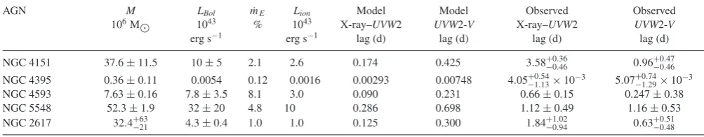
Table 3. Black hole masses, accretion rates, and resultant accretion disc model lags between the X-ray andUVW2 and between theUVW2 andVbands. For NGC 4395 both the mass and the bolometric luminosity are from Peterson et al. (2005). The masses for NGC 4151, NGC 4593, and NGC 5548 are taken from Bentz & Katz (2015) and the bolometric luminosities used in the derivation of the accretion rates are the mean and spread of observations reported by Vasudevan & Fabian (2009), Vasudevan et al. (2009,2010), and Woo & Urry (2002) The ionizing luminosity is taken from the BAT 70 month survey, extrapolated to 0.1–195 keV. Here, we assume an X-ray source height of 6Rg, an inclination of 45◦, an albedo of 0.8, and an inner disc radius of 6Rg. The observed lags for NGC 4395 are from Mc_{Hardy et al. (2016), for NGC 4151 from Edelson et al. (2017), for NGC 5548 from Edelson et al. (2015), for NGC} 2617 from Fausnaugh et al. (2018), and the results for NGC 4593 are from this work. The lags measured by Fausnaugh et al. (2018) agree, within the errors, with those presented earlier by Shappee et al. (2014). For NGC 2617, the much higher S/N 5100 Å band rather than the very nearbySwift Vband is used to measure theUVW2-Vlag. In all cases, the lags are derived from the centroid distributions using the FR/RSS method and no long-term variations have been removed from any light curve. For NGC 4395 where the observed UV band wasUVW1, the lag has been corrected to theUVW2 band assuming a scaling with wavelength to a power 1.15, which is intermediate between the expected disc value of 1.333 and the value obtained by observation which, roughly, is close to unity. For NGC 4151 and NGC 5548, X-ray lags were derived from the X4 band. For NGC 4593 where there is no evidence of variation of lag with X-ray energy, the full 0.5–10 keV band is used, as it is for NGC 4395 where the source is too faint to measure lags relative to different energy bands. For NGC 2617, we take the mass, accretion rate, and bolometric luminosity from Fausnaugh et al. (2018). The ionizing luminosity is based on the discussion of the high energy X-ray luminosity in Shappee et al. (2014). However, we note thatLionis not a critical parameter and increasing it by a factor of 3 increases the model lags by less than 1 per cent.

AGN M LBol m˙E Lion Model Model Observed Observed

106_{M 10}43 _{% 10}43 _{X-ray–UVW2 UVW2-V X-ray–UVW2 UVW2-V}

erg s−1 _{erg s}−1 _{lag (d) lag (d) lag (d) lag (d)}

NGC 4151 37.6±11.5 10±5 2.1 2.6 0.174 0.425 3.58+₋0_0..36₄₆ 0.96+₋0₀._.47₄₆ NGC 4395 0.36±0.11 0.0054 0.12 0.0016 0.00293 0.00748 4.05+₋0₁._.54₁₃×10−3 _5.07+0.74

−1.29×10−3

NGC 4593 7.63±0.16 7.8±3.5 8.1 3.0 0.090 0.231 0.66±0.15 0.247±0.38

NGC 5548 52.3±1.9 32±20 4.8 10 0.286 0.698 1.12±0.49 1.16±0.53

NGC 2617 32.4+₋63₂₁ 4.3±0.4 1.0 1.0 0.125 0.300 1.84₋+1₀._.02₉₄ 0.63+₋0₀._.51₄₈

surface of the disc may be ionized, but may be lower further out. Here, we assume an albedo of 0.8 but assuming an albedo of 0.2 only increases the median lag by 9 per cent.

We also consider only the variable component of the UV/optical emission, produced by reprocessing of high energy emission, rather than the total emission from the disc which would include emis-sion produced by dissipation of gravitational potential energy from accreting material. As the illuminating high energy emission heats the disc, the reprocessed variable emission is associated with larger radii than the same wavelength of emission from the quiescent disc. To determine how we should translate the response functions into predicted model lags we simulated aUVW2 light curve with the ob-served X-ray light curve as input. Using the FR/RSS method the measured lag using the centroids of the correlation functions was 0.131±0.024 and the lag using the peaks of the correlation func-tions was 0.076±0.03. The model median lag from the response functions is 0.096, which corresponds reasonably to the measured lags. The arrival time of the peak of the response function is typ-ically one-third of the median lag and so is much shorter than the measured lag. We therefore take the median lag of the response functions as our model lag.

5.1 Comparison of observed and modelUVW2 light curves: time-scale dependence of lags

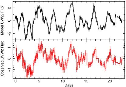
Using our disc model, with parameters given above, we can simulate the expectedUVW2 light curve, assuming illumination of the disc by the observed X-ray light curve. The resulting modelUVW2 light curve and the observedUVW2 light curve are shown in Fig.12. Fluxes are not yet included precisely in the simulation code and so the model light curve has been arbitrarily normalized to the same mean as the observed light curve. A ‘quiescent’ level of 1 mJy, which is∼0.2mJy below the lowest observedUVW2 flux was removed from theUVW2 light curve to highlight just the variable component.

0 5 10 15 20

0.2

0

.4

0.6

0

.8

Flux (mJy)

Time (days)

Figure 12. ObservedUVW2 light curve (black) with modelUVW2 light curve (red) based on a simple disc reprocessing. The normalization of the simulated light curve is arbitrary. The zero-point is the start of the intensive monitoring period.

The overall shapes of the two light curves are similar, with all of the large variations in the predicted model light curve having counterparts in the observed light curve, though the variations rel-ative to the mean level are larger in the model light curve. As has been noted by a number of previous authors (e.g. Berkley et al.

2000; Ar´evalo et al.2008), then for a lamp-post X-ray model, it is necessary to have a large X-ray source height (∼100RG) and

a similarly large inner disc radius if the amplitude and degree of smoothness of the observed UV variability are to be reproduced, assuming that all of the reprocessing is carried out on an accretion disc. We confirm that, if all of the observedUVW2 variability is to be produced by reprocessing of X-rays by just an accretion disc, then some blurring mechanism such as a large X-ray source height or scattering through the inner edge of the accretion disc (Gardner & Done2017) would be needed to reproduce the observedUVW2 amplitude of variability.

−2

0

2

Model UVW2 Flux

0 5 10 15 20

−1

0

1

Observed UVW2 Flux

Days

Figure 13. The model (upper panel) and observed (lower panel)UVW2 light curves from Fig.12following subtraction of the mean level derived from smoothing with a 5 d wide boxcar.

There are differences between the observed and model light curves in the long-term variations, e.g. with the model light curve rising in the last 5 d of the observations whereas the observed light curve continues the decrease that has been going on for the previ-ous∼15 d. Although the peaks appear to line up reasonably well, JAVELINgives a lag of the modelUVW2 by the observedUVW2 of 0.62±0.03 d, which is similar to the lag of the observed X-rays by the observedUVW2. The FR/RSS method gives a similar lag for the distribution of the centroids of the correlation functions of 0.55±0.10 d, although a shorter lag (0.28±0.12 d) for the dis-tribution of the peaks of the correlation functions. The mean peak correlation coefficient is 0.74.

If we remove the mean level derived from smoothing with a boxcar, the similarity between the remaining observed and model light curves increases, e.g. in Fig. 13 where a boxcar of width 5 d has been used. A similar relationship between the X-ray and

UVW2 light curves was also seen in NGC 5548 after long time-scale variations had been removed (fig. 5 of Mc_{Hardy et al.2014). The} similarity between the observed and model light curves indicates a strong causal relationship, as far as the short time-scale variability is concerned, between the driving X-ray light curve and the observed

UVW2 light curve. For the light curves shown in Fig.13, the lag derived byJAVELINis 0.20±0.03 d and the FR/RSS mean centroid lag is to 0.13± 0.05 d. The lags decrease as the boxcar width is reduced. With data of very high time resolution and with very short autocorrelation time-scales it might be possible to distinguish separate peaks in cross-correlation functions. However, with most real data, including the present data, the peaks are blurred together and so the effect of adding a long time-scale lag to a short time-scale lag is actually to produce a correlation function with an intermediate lag.

These results show that there are longer time-scale variations in the observedUVW2 light curve which are not reproduced by modelling by an accretion disc. However, the short time-scale (<5 d) variations can, at least to first order, be reproduced by reprocessing of the X-rays, or by some other high energy emission with similar variability properties to the X-rays, by an accretion disc. There is still some additional lag of the observedUVW2 over and above that expected from reprocessing, but it is small, and decreases as lower frequency variations are filtered out. We note that the observed lag of the unfiltered X-rays byUVW2 is ∼0.66d. This lag is much longer than might be explained by an X-ray source of size∼100RG

or a similarly large inner disc radius as, for NGC 4593,∼100RG

corresponds to 0.04d.

If the inflated inner edge of the accretion disc acts as a scatterer for the hard X-rays, adding an addition lag as in the model of Gardner & Done (2017), the fact that the X-ray to UVW2 lag becomes smaller as we remove long time-scale variations may indicate a stratified scatterer. Thus, X-rays which scatter from the top of the inflated inner disc may only undergo a small number of scatterings. They would therefore not suffer a large additional delay beyond the light traveltime expected from direct illumination of the outer disc. Similarly, the reprocessed signal in the UVOT bands should not be greatly blurred. However, X-rays which travel through a greater path-length of scatterer, along the mid-plane of the disc, will suffer longer delays and will also result in a more blurred reprocessing signal. In this model, the total UVOT light curves should be a sum of all of the reprocessed contributions.

5.2 Energetics

We can make a rough determination of whether the X-rays could be directly powering the UV/optical variations by comparing the X-ray luminosity hitting the disc, for various source geometries, and the luminosity in the varying (not the steady) component of the UV/optical fluxes. The BAT 70 month survey gives an average 14–195 keV luminosity of 1.58×1043 _{erg s}−1_{. Extrapolating to} 0.1–195 keV with=1.75 gives 3×1043_{erg s}−1_{which we take} as an approximate estimate of the total X-ray luminosity. As the lowest observed X-ray count rates are almost zero, we assume that all of the X-ray emission comes from the central varying compact source and that there is no significant quiescent component.

To estimate the total varying luminosity over the UVOT bands we have fitted models inXSPECto the data shown in Fig.11. The models are not well constrained but the total flux,∼1.16×10−11_{erg cm}−2 s−1_{over the range covered by the UVOT (∼1850−5500 Å), does} not vary by more than 10 per cent between models giving, for a distance of 35 Mpc, a luminosity of∼1.7×1042_{erg s}−1_.

To estimate the solid angle subtended at the X-ray source by the UV/optical emitting regions of the disc, we estimate, from Fig.9, that the bulk of the UV and optical emission detected by the UVOT comes from between radii of 10–300RG(1RG=38s). For an X-ray

point source at a height,H, of 6RG, this range of the disc subtends

3.22 sr, i.e. a covering fraction of 0.257 (or 0.346 forH=10RG).

Conservatively taking the lower figure gives an X-ray luminosity of 7.7×1042_{erg s}−1_{impacting the UVOT-emitting part of the disc, i.e.} about 4.5×the observed UVOT luminosity. Thus, even with a disc albedo of∼80 per cent, there would be sufficient X-ray illumination to power the observed UV/optical emission.

As an alternative way of demonstrating the energetics we show, in Fig.14the broad-band SED. The exact model fit in the UVOT bands is not important but we can see that the total luminosity in the UVOT bands does not exceed that in one decade of the X-ray spectrum.

There are, of course, a number of uncertainties in this calculation, e.g. the albedo, the X-ray source size, the illuminating X-ray energy band and the inner radius of the emission region (the outer is rela-tively unimportant). We may also wish to consider the emission at shorter wavelengths thanUVW2, but then we would have to also de-crease the inner radius which would inde-crease the solid angle. Here, we therefore conclude that, at least to first order, there is sufficient X-ray luminosity to power the observed UV/optical variations.

The above accretion disc modelling is quite basic, but serves to show that although reprocessing by an accretion disc can repro-duce a good deal of the short time-scale UV variability, there are variations on longer time-scales, with larger lags, which cannot be

0.01 0.1 1 10

10

−3

0.01

2×10

−3

5×10

−3

0.02

0.05

keV

2 (Photons cm −2 s −1 keV −1)

Energy (keV)

Figure 14. Broad-bandνF(ν) SED of NGC 4593, including the variable UVOT components, fitted to the same model as in Fig.2, together with a disc blackbody in the UVOT bands.

explained by reprocessing purely by an accretion disc. To explain all of the UV/optical variations by reprocessing of X-rays, we therefore require more than just an accretion disc as the reprocessor. Below we provide more sophisticated modelling to derive the reprocessing functions needed to reproduce all variations.

6 M E M E C H O M O D E L L I N G O F X - R AY S

D R I V I N G T H E U V A N D O P T I C A L VA R I AT I O N S

Visual inspection of the light curves and cross-correlation analy-sis indicates that a physical relationship exists between the X-ray variations and the UV/optical variations. In order to test the reality of this relationship, and to infer delay distributions rather than just mean lags for each of the UV/optical light curves, we here fit the light curves in detail, under the assumption that the X-ray variations are driving time-delayed responses in other bands.

We employed the maximum entropy fitting codeMEMECHO(Horne 1994; Horne et al.2004) to fit theSwiftlight-curve data with a

linearizedecho model

F(t|λ)=F0(λ)+ τmax

0

(τ|λ) (X(t−τ)−X0) dτ. (2)

HereX(t) is the driving (X-ray) light curve.X0is an arbitrary ref-erence level, set at the median of the X-ray data.F0(λ) is the cor-responding reference level in the echo light curve and(τ|λ) is the delay map (i.e. the response function) for the echo response at wavelengthλ.

Fig.15shows aMEMECHOfit to theSwiftlight-curve data, where

X(t) is adjusted to fit the X-ray ( 0.5–10 keV) light curve, and the reference levelsF0(λ) and delay distributions(τ|λ) are adjusted to fit the three UV light curves (UVW2,UVM2,UVW1) and the three optical light curves (U,B,V).

MEMECHOadjusts the model X-ray light curve and the echo ref-erence levels and delay maps to find a ‘good’ fit to all observed light curves, i.e. X-ray, UV, and optical, with a ‘simple’ model. The ‘good’ fit requirement is imposed on the model by requiring a specific value ofχ2_{/N, whereN= 1171 is the number of data} values. The competing requirement of a ‘simple’ model is achieved by maximizing the entropySof the functionsX(t) and(τ|λ).

We sampleX(t) and(τ|λ) on uniform grids intandτ, with the same fine spacingt=0.01 d in order to resolve the most rapid structure in the X-ray light curve. We restrict the delay map toτin the range 0–10 d, withτ >0 to impose causality (no UV/optical response prior to X-ray variations) andτ <10 d since this is roughly

1/3 of the timespan of the data and there is no sign, in the simple cross-correlations above of any strong correlation on time-scales greater than∼2 d.

The entropy of the discretely sampled positive function,p(t)=

piatt=ti, is defined as

S(p)=pi−qi−pi lnpi/qi, (3)

where for eachpithe default valueqiis the geometric mean of its

neighbours,qi=(pi−1pi+1)1/2. With this definition the entropy has a regularizing effect, expressing a preference for smooth positive functions, favouring Gaussian peaks and exponential tails. A pa-rameterWscales the entropy weight of the echo delay maps relative to that of the X-ray light curve, controlling their relative flexibility. In fitting theSwiftlight curves, we ranMEMECHOrepeatedly to find a grid of models fitting the data withχ2_{/Nranging from 2 to 0.8, and} forW=1 and 10. Here, theχ2_{level controls the trade-off between} resolution and noise in the resulting delay maps. For higherχ2_, the model light curves are too smooth to follow significant features in the light-curve data. For lower χ2 _{the model fits more subtle} features in the light-curve data, but to do so the delay maps, and to a lesser extent the model X-ray light curve, develop larger amplitude fine-scale structure that eventually, for the smallest χ2_{, becomes} unacceptable.

Fig.15presents theMEMECHOfit forχ2/N=1.5 andW=10, which we judge by eye to achieve the right balance, giving a ‘good’ fit that is not excessively ‘noisy’. Roughly speakingW=10 allows the X-ray light curveX(t) to be 10 times more flexible than the delay maps(τ|λ). This is appropriate since the most rapid structure in the X-ray light curve is not evident in the echo light curves.

Notice that the delay maps share a similar structure, with a prompt response peak atτ=0, roughly 1/4 of the response atτ <1 d, plus a broader response tail decreasing towardsτ=10 d. The extended response is generally stronger at longer wavelengths. Small bumps and wiggles on the extended response do not show a clear trend with wavelength. These may be unreliable artefacts arising from attempts to fit the echo model to residual systematic errors in the light-curve data and/or to variations that are not driven by the X-ray variations.

The fitted model adequately represents most of the features in the light-curve data, consistent with the X-ray variations driving linear responses in the UV and optical light. Evidence for the prompt response peak at 0< τ <1 d arises from many X-ray features with well-detected counterparts in the echo light curves. For example, the three X-ray dips during 7583–7585 have corresponding dips in the UV echo light curves, as do the peaks at 7599 and 7602. The more extended response is needed to produce the gradual decrease in the echo light curves.

A few minor defects in the fit may also be noted. The 1-d X-ray dip at 7590 has no counterpart in the echo light curves. The 2-d peak near 7494 in the echo light curves is well modelled, but the corresponding X-ray feature is stronger than required, so that the model X-ray light curve falls below the X-ray data in this region. In particular, the fit inserts a narrow X-ray dip in a data gap near 7594.6.

To summarize, our main conclusion is that the linearized echo model provides an acceptable fit to theSwiftlight-curve data in all wavebands. We require that the delay structure has a prompt re-sponse peak with 0< τ <1 d to produce rapid correlated variations on 1-d time-scales while washing out, from the UV/optical light curves, sub-day structure seen in the X-ray light curve. We also require an extended tail to the delay structures to produce a grad-ual decline in the UV/optical echo light curves. The rapid response

Figure 15. MEMECHOfit of the linearized echo model toSwiftlight urves of NGC 4593.Bottom panel:X-ray (0.5–10 keV) light-curve data along with the fitted modelX(t).Left column:Delay distributions(τ|λ) for three UV (UVW2,UVM2,UVW1) and three optical (U,B,V) bandpasses.Right column: Swift

light-curve data along with the echo light curves obtained by convolvingX(t) with(τ|λ). Vertical (blue) lines indicate the median (solid) and quartiles (dashed) of the delay distributions. Horizontal (red) lines indicate the reference levelsX0for the X-ray light curve andF0(λ) for the echo light curves. The fit shown is forχ2_{/N=1.5 withW=10 to makeX(t) 10 times more flexible than(τ|λ). Note the two-component structure of the delay maps, with a prompt} response peak atτ=0 and extended response reaching toτ=10 d.