The orbit and mass of the third planet in the Kepler 56 system

THE ORBIT AND MASS OF THE THIRD PLANET IN THE KEPLER-56 SYSTEM

Oderah Justin Otor1, Benjamin T. Montet2,3, John Asher Johnson3, David Charbonneau3, Andrew Collier-Cameron4, Andrew W. Howard2, Howard Isaacson5, David W. Latham3, Mercedes Lopez-Morales3,

Christophe Lovis6, Michel Mayor6, Giusi Micela7, Emilio Molinari8,9, Francesco Pepe6, Giampaolo Piotto10,11, David F. Phillips3, Didier Queloz6,12, Ken Rice13, Dimitar Sasselov3,

Damien Ségransan6, Alessandro Sozzetti14, Stéphane Udry6, and Chris Watson15 1

Department of Astrophysical Sciences, Princeton University, 4 Ivy Lane, Princeton, NJ 08544, USA;[email protected] 2

Cahill Center for Astronomy and Astrophysics, California Institute of Technology, 1200 E. California Blvd., MC 249-17, Pasadena, CA 91106, USA

3

Harvard-Smithsonian Center for Astrophysics, 60 Garden Street, Cambridge, MA 02138, USA

4

SUPA, School of Physics & Astronomy, University of St. Andrews, North Haugh, St. Andrews Fife, KY16 9SS, UK

5

Department of Astronomy, University of California, Berkeley CA 94720, USA

6

Observatoire Astronomique de l’Université de Genève, 51 ch. des Maillettes, 1290 Versoix, Switzerland

7

INAF—Osservatorio Astronomico di Palermo, Piazza del Parlamento 1, I-90134 Palermo, Italy

8

INAF—Fundacion Galileo Galilei, Rambla Jose Ana Fernandez Perez 7, E-38712 Brena Baja, Spain

9

INAF—IASF Milano, via Bassini 15, I-20133, Milano, Italy

10

Dipartimento di Fisica e Astronomia“Galileo Galilei,”Universita’di Padova, Vicolo dell’Osservatorio 3, I-35122 Padova, Italy

11

INAF—Osservatorio Astronomico di Padova, Vicolo dell’Osservatorio 5, I-35122 Padova, Italy

12

Cavendish Laboratory, J. J. Thomson Avenue, Cambridge CB3 0HE, UK

13

SUPA, Institute for Astronomy, University of Edinburgh, Royal Observatory, Blackford Hill, Edinburgh, EH93HJ, UK

14

INAF—Osservatorio Astrofisico di Torino, via Osservatorio 20, I-10025 Pino Torinese, Italy

15

Astrophysics Research Centre, Queen’s University Belfast, Belfast BT7 1NN, UK

Received 2016 August 10; revised 2016 September 17; accepted 2016 September 21; published 2016 November 15

ABSTRACT

While the vast majority of multiple-planet systems have orbital angular momentum axes that align with the spin axis of their host star, Kepler-56 is an exception: its two transiting planets are coplanar yet misaligned by at least 40°with respect to the rotation axis of their host star. Additional follow-up observations of Kepler-56 suggest the presence of a massive, non-transiting companion that may help explain this misalignment. We model the transit data along with Keck/HIRES and HARPS-N radial velocity data to update the masses of the two transiting planets and infer the physical properties of the third, non-transiting planet. We employ a Markov Chain Monte Carlo sampler to calculate the best-fitting orbital parameters and their uncertainties for each planet. Wefind the outer planet has a period of 1002±5 days and minimum mass of 5.61±0.38MJup. We also place a 95% upper limit of

0.80 m s−1yr−1on long-term trends caused by additional, more distant companions.

Key words:planets and satellites: fundamental parameters –planets and satellites: individual(Kepler-56)– techniques: radial velocities

1. INTRODUCTION

Red giant Kepler-56 (KOI-1241, KIC 6448890) is an atypical star to host transiting planets. While the vast majority of known transiting planets orbit solar-type FGK stars(Batalha et al. 2013; Burke et al. 2014; Mullally et al. 2015; Rowe et al. 2015; Grunblatt et al. 2016; Van Eylen et al. 2016), Kepler-56 is one of only a few post-main sequence stars known to host them (Lillo-Box et al.2014; Ciceri et al. 2015; Quinn et al.2015; Pepper et al.2016). Detecting transits of these stars is difficult because they are much larger than main sequence stars and have higher levels of correlated noise (Barclay et al. 2015). As such, when selecting targets for Kepler, mission scientists prioritized capturing main sequence FGK stars over other stellar types(Batalha et al.2010).

Nevertheless, Kepler-56 was targeted in the original Kepler mission (Borucki et al. 2010), and two transiting planet candidates with periods of 10.50 and 21.41 days were identified in thefirst data release(Borucki et al.2011). These candidates interacted dynamically, with observed, anticorrelated variations in their times of transit (Ford et al.2011, 2012; Steffen et al.

2012). Steffen et al.(2013)analyzed the times of transit and the orbital stability of the system to confirm these two candidates as planets, making Kepler-56 the latest stage star known at the time to host multiple transiting planets.

As a red giant, Kepler-56 exhibits convection-driven oscillations that vary on timescales long enough to be observable with Kepler long-cadence photometry. Huber et al. (2013) analyzed its observed asteroseismic modes to infer a stellar mass of 1.32±0.13M and radius of

4.23±0.15R. Through radial velocity (RV) and transit

timing observations of the transiting planets, Huber et al. (2013) then determined their masses to be 22.1-+3.63.9MÅ and

-+

181 1921MÅ, respectively. Through a combination of

asteroseis-mology and dynamical instability simulations, they also detected that the orbits of the planets, while coplanar with each other, are tilted with respect to the axis of stellar rotation by∼45°.

Huber et al.(2013)also detected the presence of a long-term RV acceleration in the data consistent with at least one additional massive companion. While the acceleration by itself cannot provide a unique orbit for the outer companion, they proposed that both the planetary obliquity and long-term RV trend could be explained by a non-transiting companion with a period of 900 days and mass 3.3MJup.

any confirmed planet orbiting aKeplerstar(Kostov et al.2015; Kipping et al.2016). We are also able to place upper limits on the presence of additional planets from the lack of additional long-term trends in the RV curve.

In Section2we describe our data collection and reduction. In Section3, we describe our RV model. In Section4, we present our best estimates for this planet’s orbital parameters, as well as the likelihood of another companion. We discuss our results in Section 5and summarize ourfindings in Section6.

2. DATA COLLECTION AND ANALYSIS

Our analysis is based on 43 RV observations of Kepler-56 obtained from 2013 to 2016 with two different spectrographs: 24 with Keck/HIRES(Vogt et al.1994)and 19 with HARPS-North(Cosentino et al.2012).

2.1. Keck/HIRES Observations

Our Keck/HIRES observations were obtained largely following the standard procedures of the California Planet Survey(CPS)team(Howard et al.2010), modified slightly for the faint stars of the Kepler field, following the approach of Huber et al. (2013). For all observations, we used the C2 decker(14 0×0 85), which is a factor of four taller than the B5 decker typically used for observations of bright stars. This setup allows for more background light to enter the spectro-graph, allowing for better sky subtraction while maintaining a resolving power of R≈50,000.

Each observation was made with an iodine cell mounted along the light path before the entrance to the spectrograph. The iodine spectrum superposed on the stellar spectrum provides a precise, stable wavelength scale and information on the shape of the instrumental profile of each observation (Valenti et al.1995; Butler et al.1996).

The integration times range from 600 to 1800 s. The star-times-iodine spectrum was modeled using the Butler et al. (1996)method, with the instrumental profile removed through numerical deconvolution. The RV of the star at each observation is compared to a template spectrum of the star obtained without iodine, with the instrumental profile removed through numerical deconvolution. The observed RVs are listed in Table1.

The data set used here includes the 10 observations used by Huber et al. (2013), re-analyzed after all observations were recorded. An improved stellar template spectrum causes the measured RV from these observations to be slightly different than those reported by Huber et al. (2013), although the differences are smaller than the formal uncertainties on each observation.

2.2. HARPS-North Observations

We also obtained 19 observations of Kepler-56 with HARPS-North, a high-precision echelle spectrograph at the 3.6 m Telescopio Nazionale Galileo(TNG)at the Roque de los Muchachos Observatory, La Palma, Spain. HARPS-N is a

fiber-fed high-resolution(R=115,000)spectrograph optimized for measuring precise RVs.

The exposure times for all observations with HARPS-N were 1800 s, and the data were reduced with version 3.7 of the standard HARPS-N pipeline. RVs were derived with the standard weighted cross-correlation function method (Baranne

et al. 1996; Pepe et al. 2002). These data are also listed in Table1.

Note that the HARPS-N pipeline includes the systemic RV, while the Keck/HIRES pipeline does not, leading to a 54.25 km s−1apparent shift between the two sets.

3. ORBIT FITTING

With the RV data in hand, we can determine the orbital parameters of the outer planet. We develop code that, for a given set of orbital parameters, returns the expected RV contribution from each planet at a list of user-specified times following Lehmann-Filhés(1894)and Eastman et al.(2013).

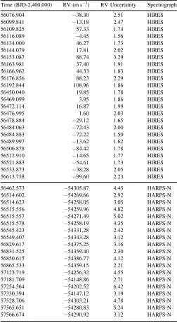
Table 1

RV Observations of Kepler-56

Time(BJD-2,400,000) RV(m s−1) RV Uncertainty Spectrograph

56076.904 −38.30 2.51 HIRES

56099.841 −13.18 2.47 HIRES

56109.825 57.33 1.74 HIRES

56116.089 −4.45 1.56 HIRES

56134.000 46.27 1.73 HIRES

56144.079 17.81 2.02 HIRES

56153.087 88.74 3.29 HIRES

56163.981 37.40 1.91 HIRES

56166.962 44.33 1.83 HIRES

56176.856 88.23 2.29 HIRES

56192.844 108.96 1.86 HIRES

56450.040 19.85 1.78 HIRES

56469.099 3.95 1.86 HIRES

56472.114 16.87 1.99 HIRES

56476.995 1.60 2.03 HIRES

56478.884 −29.12 1.65 HIRES

56484.063 −72.43 2.00 HIRES

56484.883 −72.22 1.50 HIRES

56489.997 −13.62 1.62 HIRES

56506.878 −84.42 1.78 HIRES

56512.910 −14.65 1.77 HIRES

56521.883 −54.61 1.73 HIRES

56533.873 −38.28 2.05 HIRES

56613.758 −99.60 2.23 HIRES

56462.573 −54305.87 4.45 HARPS-N 56514.602 −54269.66 2.92 HARPS-N 56514.623 −54258.05 3.05 HARPS-N 56515.556 −54259.96 4.82 HARPS-N 56515.557 −54271.49 5.02 HARPS-N 56515.578 −54258.19 4.35 HARPS-N 56545.423 −54331.28 2.42 HARPS-N 56549.407 −54343.28 3.12 HARPS-N 56829.617 −54375.25 3.16 HARPS-N 56831.525 −54359.40 2.30 HARPS-N 56850.615 −54386.77 4.12 HARPS-N 56865.533 −54359.15 2.21 HARPS-N 57123.719 −54256.32 4.55 HARPS-N 57181.709 −54148.86 2.71 HARPS-N 57254.564 −54202.52 6.42 HARPS-N 57330.394 −54147.12 3.19 HARPS-N 57528.706 −54303.21 4.78 HARPS-N 57565.651 −54280.83 5.24 HARPS-N 57566.674 −54290.92 3.12 HARPS-N

Our algorithm does not include variations caused by dynamically interacting planets. However, Kepler-56 b’s RV signal is small relative to our RV precision and the magnitude of Kepler-56 c’s perturbation is small relative to its orbital period, so we do not expect to see any perturbation signal in the data. The two spectrograph pipelines return different RV offsets, so we make an initial guess for the relative offset between the two in ourfitting.

For each planet, we include the minimum mass (msini), including the unknown inclination of the non-transiting planet, and two vectors that define the eccentricity and argument of periastron ( ecosw and esinw), following Eastman et al.(2013).

For the outer planet alone, we include the orbital period(P) and time of transit (ttr, if it were so aligned); these values are

fixed for the inner planets. The stellar mass (M), separate instrumental offsets(γ), and RV jitter terms(σjitter)for HARPS and HIRES complete our list of parameters. Functionally, as the HARPS pipeline returns a measurement with the systemic RV included (ignoring features like the gravitational redshift and convective blueshift), the offset associated with that instrument approximates the true systemic velocity of the star while the offset for HIRES brings these two sets of observations onto the same scale.

We only consider models of three planets plus a long-term RV acceleration. While it is possible that two planets in circular orbits with orbital periods near a 2:1 period ratio can

masquerade in RV observations as a single planet with a higher eccentricity (Anglada-Escudé et al. 2010), there is no evidence that such an effect is occurring in our data set. However, we lack the phase coverage to fully rule out this hypothesis. More observations where our coverage is sparse would be helpful to probe for a fourth planet in resonance with the third.

After solving Kepler’s equation to obtain the Keplerian orbital elements, the function produces radial velocities following

⎜ ⎟

⎛

⎝ ⎞⎠ 

p

q w w w

= + -´ + + G P m i

M m _e

e t t e

RV 2 sin 1

1

cos , , , cos . 1

1 3

2 3 ₂

obs obs

( )

[ ( ( ) ) ] ( )

Here, θ represents the true anomaly,tobs is its specific value, andωis the argument of periastron.

With our function’s ability to generate an RV curve for any specified period, we can test various combinations of the outer companion’s orbital parameters. We exploit this ability in performing successivefits to obtain an initial estimate of our planetary parameters.

3.1. Maximum Likelihood Estimation

First, we perform maximum likelihood estimation via Python’s scipy.optimize.minimize routine. For the possible companion, we take all values as unknown. Specifi -cally, wefit for ecosw, esinw,msini,P,M,ttr, andg˙, the acceleration of the entire system over time. Since our measurements come from two instruments, we include independent offset terms for each, γHARPS and γHIRES, where γis the systemic RV offset term introduced in Section3. There are 17 free parameters in total—these, plus ecosw, ecosw, andmsini for each planet(as mentioned in Section3).

Maximum likelihood estimation is a process in which we calculate the logarithm of likelihood(L)by comparing our data (D)to the sum of our generated RV curves through the standard equation ⎛ ⎝ ⎜ ⎞ ⎠ ⎟

å

= - - - +

L D N

ln 1

2

RV 1

2 ln 2 2

i N i i i i 1 jitter, 2 jitter, 2 ( ) ( ) ( )

sjitter,i=si +j . 3

2 2 2 _{( )}

We useσjitterin order to incorporate jitter. Sources of jitter include uncertainties in measurements beyond photon noise that arise from sources like noise in the detector or stellar activity. For sub-giant stars, typical jitter values are 3–5 m s−1 (Johnson 2008). Given the longer exposures for this star relative to previous studies of planets around relatively bright subgiants, we might expect a lower level of jitter as the integrations will average over the higher-order modes.

We initialize the fit with values from Huber et al. (2013). However, we note a typo in Table 1 of the discovery paper: the listed times of transit in that paper are too large by 20 days. They should be 2454958.2556 and 2454958.6560 days for Kepler-56 b and c, respectively, rather than 2454978.2556 and 2454978.6560 days.

We reject trials with nonphysical results such as negative masses and periods. For steps that are not rejected, we apply normal priors with expected values and 1σuncertainties based on measurements from Huber et al.(2013)for the asteroseismic mass of the host star and the inner planets’ photodynamical

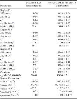
Table 2

Orbital Parameters for the Kepler-56 System

Parameters

Maximum like-lihood Best-fits

emceeMedian Fits and 1σ Uncertainties

Kepler-56 b

w

e1cos 1 0.20 0.19±0.04

w

e1sin 1 −0.04 −0.04±0.05

e1 a

0.04 0.04±0.01 ω1(Radians)

a

−0.20 −0.19±0.29 M1sini1(MÅ) 29.4 30.0±6.2 Kepler-56 c

w

e2cos 2 −0.00 −0.01±0.09

w

e2sin 2 −0.12 −0.05±0.04

e2a 0.01 0.00±0.01

ω2(Radians)a −1.61 −1.70±1.46

M2sini2(MÅ) 191 195±14

Kepler-56 d

w

e3cos 3 0.44 0.44±0.03

w

e3sin 3 −0.12 −0.12±0.04

e3 a

0.21 0.20±0.01 ω3(Radians)

a

−0.27 −0.26±0.10 M3sini3(MÅ) 1767 1784±120

M3sini3(MJup) 5.55 5.61±0.38

P3(days) 1002 1002±5

ttr,3(BJD-2,400,000) 56449 56450±7

System Parameters

g˙ (m s−1yr−1) −0.26 −0.25±0.33

g_HARPS(m s−1) −54276.1 −54276.2±2.0 γHIRES(m s−1) −27.7 −27.7±2.0 sjitter,HARPS(m s−1) 0.72 1.23±0.466

sjitter,HIRES(m s−1) 1.68 1.80±0.179

Note.

a

eccentricity vectors, based on the TTV analysis of the Kepler light curve. The sum of the logarithm of each prior term is saved for each set of parameters that is tested.

Then, we calculate the logarithm of the posterior probability for each model, which is the sum of the prior and log-likelihood terms(as maximizing the logarithm of a function is equivalent to maximizing the function itself). Equation (4)

illustrates this process:



= +

p L D

ln RV D ln ln RV . 4

N

[ ( ∣ )] [ ( )] [ ( ∣ )] ( )

Equation (4) calculates the logarithm of the posterior probability distribution function for any set of model parameters (q) as compared to our RV data (D). The combination of parameters found by this process to make the data most probable then becomes the initial guess for ourfinal

fitting process.

3.2. Markov Chain Monte Carlo Analysis

We use the result of maximum likelihood estimation from Section 3.1as the initialization foremcee (Foreman-Mackey et al. 2013), a Markov Chain Monte Carlo (MCMC) implementation for Python of the affine-invariant ensemble sampler of Goodman & Weare(2010).

Our 17 parameter simulation uses 150 walkers and 6000 steps, with an observed burn-in of 1500 steps.

4. RESULTS

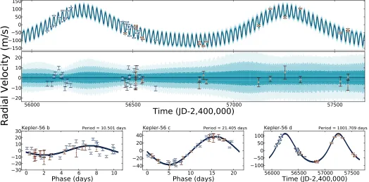
We detect a massive, non-transiting companion, designated Kepler-56 d, withfinal best-fit values and uncertainties listed in

Table 2. The RV curve generated by our highest-confidence combination of parameters can be seen in tandem with its uncertainties and our original RV data in Figure1. In the same

figure, we also show the maximum likelihood orbits for each individual planet as well as the data with the maximum likelihood signals from the other two planets removed. These data are only for visualization purposes; at all times wefit the contributions from all three planets simultaneously.

For Kepler-56 d itself, we return a Doppler semi-amplitude of 95.21±1.84 m s−1, corresponding to a minimum mass of 5.61±0.38MJup (1784±120MÅ). We also measure a period

of 1002±5 days, an eccentricity of 0.20±0.01, and a semimajor axis of 2.16±0.08 au.

4.1. Limits on a Fourth Planet

A fourth planet beyond the orbit of Kepler-56 d, if it exists, could be observable through the detection of a long-term trend in the data. Given our three-year baseline of observations, we can place limits on the presence of such an outer companion. From ouremceeresults, wefind a long-term RV acceleration of −0.25±0.32 m s−1yr−1. The 95th percentile value of the

emcee posterior probability distribution for g˙ provides an upper limit on acceleration from a fourth planet of 0.80 m s−1yr−1.

From Montet et al. (2014), we know the maximum trend caused by a planetary companion on a circular orbit is

⎜ ⎟

⎛ ⎝

⎜ ⎞

⎠ ⎟⎛_⎝ ⎞_⎠

g= - - m i

-M

a

6.57 m s yr sin

5 au , 5

p

1 1 Jup

2

˙ ( ) ( )

where mpis the mass of the planet,MJupthe mass of Jupiter, andathe orbital semimajor axis. From this, we can place limits on the presence of outer companions with msini larger than 0.49MJup at 10 au and 1.95MJup at 20 au; such companions must be at particular points in their orbits or at low inclination in order to evade RV detection.

At V;13 mag, Kepler-56 falls just within Gaiaʼs bright-star limit(Perryman et al.2014). A fourth planet’s acceleration on Kepler-56 in Gaia astrometry might be detectable at the level of 10–20μas yr−2 over the course of the mission. Averaging over flat priors for orbital angles and eccentricity, at the nominal distance of Kepler-56(d∼850 pc),Gaiacould in principle detect curvature due to orbital motion of a companion of20MJupat 10 au or 80MJupat 20 au. These values in Equation(5)return, at the lowest, an acceleration of 32.85 m s−1yr−1. This is much higher than the limits returned by ourfit, suggesting that, save for face-on orbits,Gaiawill be less helpful than continued RV observation in placing further limits on a fourth planet.

A fourth planet in a near-resonant orbit with Kepler-56 d could masquerade as a single eccentric planet, as described by Anglada-Escudé et al.(2010). However, wefind the probability of this scenario to be low. Re-running ouremcee fit with the outer planet’s eccentricity fixed at 0 leads to decreased likelihoods for the fit as a whole, and we do not detect any long-term structure in the residuals. However, our observations do not have the time resolution necessary to make a definitive assertion on this effect. Complete phase coverage of Kepler-56 d is needed to answer this question.

5. DISCUSSION

5.1. Comparison to Previous Work

Our research supports that of Huber et al.(2013)infinding strong evidence for a massive, non-transiting exoplanet in the Kepler-56 system. Now that our observations span a full Kepler-56 d orbit, we can compare our results with the projections from Huber et al.(2013), who predicted that both the planetary obliquity and long-term RV trend could both be broadly explained by a non-transiting companion with a period of 900 days and mass of 3.3MJup.

Both our minimum mass and period are similar to the representative values listed by Huber et al. (2013). Kepler-56 d’s minimum mass could be commensurate with that of a giant planet or a brown dwarf(for inclinations below 30°). This could have implications for the near 2:1 resonance of the inner planets’orbits, as well as for the misalignment of their orbital plane with that of Kepler-56ʼs rotation. Indeed, Li et al.(2014)

simulated several scenarios and found a higher probability of the observed misalignment being of a dynamical origin (e.g., Fabrycky & Tremaine2007)than from migration of the bodies in a tilted protoplanetary disk(e.g., Bate et al.2010)or through angular momentum transport in the star itself that led to an apparent misalignment, even if the system was originally aligned(Rogers et al.2012).

While Kepler-56 d is a possible source of dynamical perturbation, Gratia & Fabrycky (2016, submitted) simulate the scattering of two giant outer planets and find scattering between a system of three outer planets is required to excite the two inner planets of the system to inclinations similar to those observed in the data while preserving coplanarity. These additional planets, if real, must be scattered to large orbital

separations or ejected entirely to evade detection by our RV observations.

5.2. The Effect of Kepler-56 d on Transits of the Inner Planets

Huber et al. (2013) inferred masses of the system’s inner planets by dynamically modeling their transits, ignoring possible perturbations from the third, outer planet. We verify that this is a reasonable assumption by checking two effects that may be significant: a tidal term corresponding to the change in the gravitational potential as Kepler-56 d completes its orbit, and a Roemer delay as the distance to the inner planets and host star varies over the orbit of the outer planet.

Following Equations(25)–(27) of Agol et al. (2005), the tidal effects would cause, over a long time baseline, the transits of an inner planet with massm1and periodP1to be perturbed with a standard deviation

⎡

⎣⎢ ⎤⎦⎥

s= b

-´ - -

-e

e

e e e

3 2 1

1 3

16

47 1296

413

27648 , 6

2

22 3 2

2 2

2 4

2 6 1 2

( )

( )

wheree2is the eccentricity of the outer planet and

b p

=

+ m

m m

P P

2 . 7

2

0 1 1

2

2

( ) ( )

Here,m2is the mass of the outer planet with orbital periodP2, andm0the mass of the host star.

For the values in Table 2 for our system, we find perturbations in the time of transit on the order of 4 s for Kepler-56 b and 16 s for Kepler-56 c. Given that the precision in the measurement of times of transit of these planets is typically tens of minutes, we do not expect these perturbations to affect, or be noticeable in, the measured times of transit.

The light travel time, or Roemer, delay is the result of changes in the physical distance between the observer and the host star due to the orbit of the outer body. Following Equations(6)and(7)of Rappaport et al.(2013), its magnitude is bounded such that

⎡ ⎣⎢

⎤ ⎦⎥



p + +

A G

c P

m i

m m m

2

sin

, 8

R

1 3

2 3 2

2 3 2 2

0 1 22 3

( ) ( ) ( )

where G is Newton’s constant, c the speed of light, and all other terms retain their meaning from the previous equation. Inserting values from Table2again, wefind the expected light travel time signal not to exceed 5 s, significantly smaller than the observed uncertainties, so we do not expect Kepler-56 d to affect the orbits of the inner planets in any observable way.

5.3. Alternative Methods of Measuring Kepler-56 d

posterior distribution of the time of central transit. The transit duration allows us to place even tighter constraints. If Kepler-56 d transited with an impact parameter b=0, the transit would have a duration of 3.1 days. As none of the gaps are longer than 20 hr in duration, we can additionally rule out any transits withb<0.95. By again integrating over the posterior distribution but accounting for the nonzero transit duration, assuming a flat distribution in impact parameter, we find that only 0.07% of allowed transits fall fully inside a data gap. If Kepler-56 d were to transit, there is a 99.93% proabability it would be observable in the Kepler data. Given this low probability and the a priori small transit probability for a companion on a∼1000 day period, it is likely this companion is non-transiting. We note that non-transiting does not necessarily imply non-coplanarity with the inner planets, as the transit probability decreases with increasing semimajor axis (Borucki & Summers1984).

Having measured the minimum mass (msini) and orbital semimajor axis (a) of Kepler-56 d, we can consider the possibility that theGaiaastrometric mission would be able to constrain its inclination. For lower(more face-on)inclinations, the planet will have a higher mass and the center of mass of the system will move closer to the planet. Additionally, the astrometric orbit will change shape on the sky, with more face-on inclinatiface-ons appearing more circular throughout an orbit.

Given the distance to the system (d∼850 pc) and the inferred semimajor axis 2.13±0.07 au, the orbit of Kepler-56 d has a projected semimajor axis on the sky of ∼2.5 mas. From the mass ratio between the planet and star, we then expect an astrometric signal with a semi-amplitude of 11 sin-1 _μas.

Perryman et al.(2014)determined thatGaiawill detect planets with astrometric signatures larger than 68μas for stars as bright as Kepler-56, meaning this planet would evade detection at all except the lowest inclinations. However, given that the Gaia data can be combined with the prior information about the orbit of Kepler-56 d from RVs, it may be possible that the planet will be detected at slightly lower inclinations. Regardless, the prospects of a robust determination of the outer planet’s complete set of orbital parameters from Gaiaappear unlikely.

6. SUMMARY

Kepler-56, a red giant targeted in the telescope’s primary mission, has a massive, non-transiting companion detected through radial velocities. This star is one of only a few red giants known to have transiting planets, and these planets orbit with a nearly 2:1 period ratio on a plane misaligned relative to the spin of their host star. The presence of another body in the system was first detected by Huber et al. (2013) with observations from Keck/HIRES; we follow them up with subsequent observations from HIRES and HARPS-North at TNG. Incorporating these new data, we model the RV curve for a three-planet system. Our results confirm the existence of Kepler-56 d, with a period of 1002±5 days and a minimum mass of 5.61±0.38MJup. We also return an upper limit of

acceleration from a possible fourth planet of 0.80 m s−1yr−1at 95% confidence, severely restricting the possibility of the existence of other giant planets within ∼20 au. We find that Kepler-56 d should not be detectable through its dynamical effect on the transits of the two inner planets, but for sufficiently face-on(more massive)orbits could be detectable through Gaiaobservations of its astrometric wobble.

We thank Eric Agol, Daniel Fabrycky, and Daniel Huber for comments and conversations which improved the quality of this manuscript.

O.J.O. thanks the members and friends of the Banneker Institute, who made the summer in which this project began a fruitful time. He also thanks Neta Bahcall for allowing him to continue this research as his senior thesis. He gratefully acknowledges support from the Banneker Institute and Princeton’s astrophysics department, Class of 1984, and Office of the Dean of Undergraduate Students in facilitating travel to AAS 227 to present this research. He would be remiss to forget the other members of the Party of Three and their associates.

B.T.M. is supported by the National Science Foundation Graduate Research Fellowship under Grant No. DGE1144469. J.A.J. is supported by generous grants from the David and Lucile Packard Foundation and the Alfred P. Sloan Foundation. C.A.W. acknowledges support from STFC grant ST/ L000709/1.

This publication was made possible through the support of a grant from the John Templeton Foundation. The opinions expressed in this publication are those of the authors and do not necessarily reflect the views of the John Templeton Founda-tion. This material is based upon work supported by the National Aeronautics and Space Administration under grant No. NNX15AC90G issued through the Exoplanets Research Program.

The research leading to these results has received funding from the European Union Seventh Framework Programme (FP7/2007-2013) under Grant Agreement No. 313014 (ETAEARTH).

Some of the data presented herein were obtained at the W.M. Keck Observatory, which is operated as a scientific partnership among the California Institute of Technology, the University of California and the National Aeronautics and Space Adminis-tration. The Observatory was made possible by the generous

financial support of the W.M. Keck Foundation. The authors wish to recognize and acknowledge the very significant cultural role and reverence that the summit of Maunakea has always had within the indigenous Hawaiian community. We are most fortunate to have the opportunity to conduct observations from this mountain.

The HARPS-N project was funded by the Prodex program of the Swiss Space Office (SSO), the Harvard University Origin of Life Initiative (HUOLI), the Scottish Universities Physics Alliance (SUPA), the University of Geneva, the Smithsonian Astrophysical Observatory (SAO), and the Italian National Astrophysical Institute (INAF), University of St. Andrews, Queens University Belfast, and University of Edinburgh.

Facilities:Keck:I(HIRES), TNG(HARPS-N).

REFERENCES

Agol, E., Steffen, J., Sari, R., & Clarkson, W. 2005,MNRAS,359, 567

Anglada-Escudé, G., López-Morales, M., & Chambers, J. E. 2010, ApJ,

709, 168

Baranne, A., Queloz, D., Mayor, M., et al. 1996, A&AS,119, 373

Barclay, T., Quintana, E. V., Adams, F. C., et al. 2015,ApJ,809, 7

Batalha, N. M., Borucki, W. J., Koch, D. G., et al. 2010,ApJL,713, L109

Batalha, N. M., Rowe, J. F., Bryson, S. T., et al. 2013,ApJS,204, 24

Bate, M. R., Lodato, G., & Pringle, J. E. 2010,MNRAS,401, 1505

Borucki, W. J., Koch, D., Basri, G., et al. 2010,Sci,327, 977

Borucki, W. J., Koch, D. G., Basri, G., et al. 2011,ApJ,736, 19

Borucki, W. J., & Summers, A. L. 1984,Icar,58, 121

Burke, C. J., Bryson, S. T., Mullally, F., et al. 2014,ApJS,210, 19

Ciceri, S., Lillo-Box, J., Southworth, J., et al. 2015,A&A,573, L5

Cosentino, R., Lovis, C., Pepe, F., et al. 2012,Proc. SPIE,8446, 84461V

Eastman, J., Gaudi, B. S., & Agol, E. 2013,PASP,125, 83

Fabrycky, D., & Tremaine, S. 2007,ApJ,669, 1298

Ford, E. B., Fabrycky, D. C., Steffen, J. H., et al. 2012,ApJ,750, 113

Ford, E. B., Rowe, J. F., Fabrycky, D. C., et al. 2011,ApJS,197, 2

Foreman-Mackey, D., Hogg, D. W., Lang, D., & Goodman, J. 2013,PASP,

125, 306

Goodman, J., & Weare, J. 2010,Communications in Applied Mathematics and Computational Science, 5, 65

Gratia, P., & Fabrycky, D. C. 2016, MNRAS, submitted

Grunblatt, S. K., Huber, D., Gaidos, E. J., et al. 2016, arXiv:1606.05818

Howard, A. W., Johnson, J. A., Marcy, G. W., et al. 2010,ApJ,721, 1467

Huber, D., Carter, J. A., Barbieri, M., et al. 2013,Sci,342, 331

Johnson, J. A. 2008, in ASP Conf. Ser. 398, Extreme Solar Systems, ed. D. Fischer et al.(San Francisco, CA: ASP),59

Kipping, D. M., Torres, G., Henze, C., et al. 2016,ApJ,820, 112

Kostov, V. B., Orosz, J. A., Welsh, W. F., et al. 2015, arXiv:1512.00189

Lehmann-Filhés, R. 1894,AN,136, 17

Li, G., Naoz, S., Valsecchi, F., Johnson, J. A., & Rasio, F. A. 2014,ApJ,

794, 131

Lillo-Box, J., Barrado, D., Moya, A., et al. 2014,A&A,562, A109

Montet, B. T., Crepp, J. R., Johnson, J. A., Howard, A. W., & Marcy, G. W. 2014,ApJ,781, 28

Mullally, F., Coughlin, J. L., Thompson, S. E., et al. 2015,ApJS,217, 31

Pepe, F., Mayor, M., Rupprecht, G., et al. 2002, Msngr,110, 9

Pepper, J., Rodriguez, J. E., Collins, K. A., et al. 2016, arXiv:1607.01755

Perryman, M., Hartman, J., Bakos, G. Á., & Lindegren, L. 2014, ApJ,

797, 14

Quinn, S. N., White, T. R., Latham, D. W., et al. 2015,ApJ,803, 49

Rappaport, S., Deck, K., Levine, A., et al. 2013,ApJ,768, 33

Rogers, T. M., Lin, D. N. C., & Lau, H. H. B. 2012,ApJL,758, L6

Rowe, J. F., Coughlin, J. L., Antoci, V., et al. 2015,ApJS,217, 16

Steffen, J. H., Fabrycky, D. C., Agol, E., et al. 2013,MNRAS,428, 1077

Steffen, J. H., Ford, E. B., Rowe, J. F., et al. 2012,ApJ,756, 186

Valenti, J. A., Butler, R. P., & Marcy, G. W. 1995,PASP,107, 966

Van Eylen, V., Albrecht, S., Gandolfi, D., et al. 2016, arXiv:1605.09180