doi:10.4236/iim.2010.211072 Published Online November 2010 (http://www.SciRP.org/journal/iim)
Record Values from the Inverse Weibull Lifetime Model:
Different Methods of Estimation
Khalaf S. Sultan
Department of Statistics and Operations Research, College of Science, King Saud University, Riyadh, Saudi Arabia E-mail: [email protected]
Received September 21, 2010; revised October 13, 2010; accepted November 15,2010
Abstract
In this paper, we use the lower record values from the inverse Weibull distribution (IWD) to develop and discuss different methods of estimation in two different cases, 1) when the shape parameter is known and 2) when both of the shape and scale parameters are unknown. First, we derive the best linear unbiased estimate (BLUE) of the scale parameter of the IWD. To compare the different methods of estimation, we present the results of Sultan (2007) for calculating the best linear unbiased estimates (BLUEs) of the location and scale parameters of IWD. Second, we derive the maximum likelihood estimates (MLEs) of the location and scale parameters. Further, we discuss some properties of the MLEs of the location and scale parameters. To compare the different estimates we calculate the relative efficiency between the obtained estimates. Finally, we propose some numerical illustrations by using Monte Carlo simulations and apply the findings of the paper to some simulated data.
Keywords:Scale Parameter, Location Parameter, Best Linear Unbiased Estimates (BLUEs), Maximum Likelihood Estimates, Relative Efficiency and Monte Carlo Simulations
1. Introduction
Record values arise naturally in many real life applications involving data relating to weather, sport, economics and life testing studies. Many authors have studied record values and the associated statistics; see, for example, [1-7]. Reference [8] has established some recurrence relations for the moments of record values from the Gumbel distribution. Similar work has been carried out by [9,10] for the generalized extreme value and exponential distributions, respectively. Reference [11] have also discussed some inferential methods based on record values from Gumbel distribution. [12,13] have discussed inferential techniques based on Weibull and generalized Pareto distributions, respectively. Reference [14] have compared different estimates based on record values from Weibull distribution. Reference [15] has considered different loss functions to develop the Bayesian estimates of the parameters of the IWD.
Let XL(1),XL(2),,XL n( ) be the first n lower record values from the IWD with density function
(pdf)
1
( ) = c x c, 0, > 0,
f x cx e x c (1.1)
and cumulative distribution function (cdf )
( ) = x c, 0, > 0.
F x e x c (1.2) The scale form of the IWD has its density function given by
1exp , 0, > 0c c
c
f y y
y y
(1.3)
while the location-scale IWD has its density function given by
1exp , 0, > 0, 0c c
c
f y y
y y
(1.4) Reference [16] calls the IWD as the complementary Weibull distribution, while [17] call it the reciprocal Weibull distribution. Reference [18] have discussed some useful measures for the IWD.
Reference [20] has fitted the IWD to the flood data. For more details on the IWD, see for example, [21].
The joint density function of the first n lower record values XL(1),XL(2),,XL n( ) is given by [5]
1 ( ) 1,2, , (1) (2) ( ) ( )
=1 ( ) ( )
( , , , ) = ( ) .
( )
n L i
n L L L n L n
i L i
f x
f x x x f x
F x
(1.5)
From (1.5), the pdf. of XL m( ) can be obtained as
11
( ) = log[ ( )] ( ), 0, = 1, 2, , ( )
m m
f x F x f x x m
m
(1.6) where f(.) and F(.) are given in (1.1) and (1.2), respectively.
The the joint pdf of XL m( ) and XL n( ) is given by
1 ,1
( , ) = log[ ( )] { log[ ( )] ( ) ( )
m m n
f x y F x F y
m n m
1 ( )
log[ ( )]} ( ) , 0 < < , ( )
, = 1, 2, , < , n m f x
F x f y y x
F x
m n m n
(1.7)
where f(.) and F(.) are given in (1.1) and (1.2), respectively.
The single and product moments of record values are (see [22])
( )
( )
= , < ,
( )
i m
i m
c i mc m
(1.8) and
( , ) ,
( ) ( )
= , < , < ,
( ) ( ) i j
m n
i i j
m n
c c i j nc m n
i m n c
(1.9)
where ( ) is the gamma function.
In the following section, we derive the exact form of the BLUE scale parameter and present the BLUEs of the location-scale case of IWD. Next in Section 3, we derive the maximum likelihood estimates of the parameters of IWD. Finally, in Section 4 we discuss the relative efficiency of the obtained estimates.
2. The BLUEs
In this section, we derive the BLUE of the scale parameter and present the BLUEs of the location and scale parameters of the IWD.
2.1. The Scale Case
Let YL(1),YL(2),,YL n( ) denote the first n lower record
from the distribution in (1.3), and let
( )= ( )/ , = 1, 2, , L i L i
X Y i n be the corresponding
record values from the IWD in (1.1). Assume
1, 2, ,
,T
L L L n
Y Y Y Y
1, 2, ,
T n
1 1,1, 1T
n
and
, , 1 , i j i j n
. Then, the BLUE of thescale parameter is given by 1
*
1 1 ( )
=1
= = ,
T n
i L i T
i
Y a Y
(2.1) and its variance is given by* 2
1 1
1
( ) = T ,
Var
(2.2)
for details, refer to [23,6]. Since the double moment
, m n
can be written as
,
( 1 / )
= , =
( ) ( 2 / ) ( 1 / )
= , > 2 / ,
( 1 / ) ( )
m n m n m
n
m c
p q p and
m
n c n c
q n c
n c n
(2.3)
then the covariance matrix can be inverted analytically. Then ( , )i j th element ijof 1 can be derived as
2 2 2 2
2
1
=
( 1) ( 1)
, = 1, = 1, 2, , 1, ( 2 / )
(2 2 4 2 1) ( )
= = 2 1 ( 2 / )
( 1)
, = = 1, (1 2 / )
( 1) ( )
, = = ( 1 2 / )
0, > 1. ij
n
n
c ic i
j i i n
i c
i c ic ic c c i
i j and n
i c
c
i j c
q c nc c n
i j n
q n c
j i , , (2.4) From (1.8), (2.1) and (2.4), we have the BLUE of the scale parameter as
*
1 ( ) ( )
( )
= = ,
( 1 / )
n L n L n
n
a y Y
n c
(2.5)
with variance is given by
2
* 2
1 2
( ) ( 2 / ) ( 1 / )
( ) = , n 2 / c.
( 1 / )
n n c n c
Var n c (2.6) It is clear from (2.5) that *
.
Table 1 below shows the coefficients
a
n of the BLUE of when n= 4 to 7 and = 3, 4, 5c .The BLUE of given in (2.5), can be used to construct 100(1)% confidence interval for through the formula
* *
1 1
1 / 2 / 2
( 1 / ) ( 1 / )
1 ,
( ) ( )
n c n c
P
n T n T
(2.7)
where T/ 2 and T1/ 2 are the lower and upper percentage points of the pivotal quantity
*
1 ( 1 / )
= .
( )
n c
T
n
The cdf of T is obtained to be ( ) = ( , ), ( )
c T
n t F t
n
where ( ,n tc) is the incomplete gamma function. Example
Five lower record values are simulated from IWD with
= 3
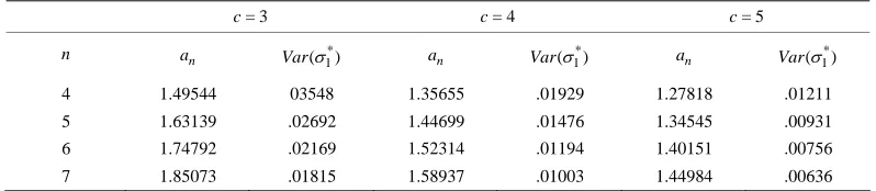
c and = 1.0 as follows: 3.07586, .90607, 68454, .62296, .62283, by using the coefficients of the BLUE of the scale parameter given in Table 1, we have
*
1 = 1.63139(.62283) = 1.016079,
and the standard
error of this estimate is S E. .(1*) =1.016079 .02692 = 0.166711. Now, we calculate the lower and upper
5% percentage points of of T to be
0.025 = 0.46048001250
T a n d T0.975 = 0.8508449965 .
Then 95% confidence interval for can be calcu- lated from (2.7) to be (0.7320149148 , 1.352569185).
2.2. The location-Scale Case
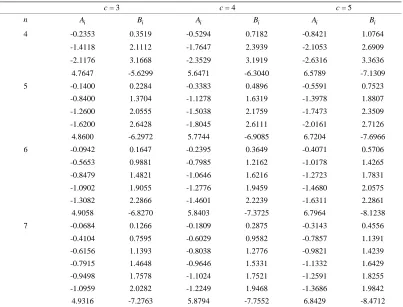
Reference [15] has used the single and product moments of the record values from IWD. Then, he has used these moments to calculate the coefficients of BLUEs and the variances for records of size 4,5,6 and 7 and c= 3, 4, 5
by using the forms (see [23]).
* *
2 ( ) 2 ( )
=1 =1
= , = .
n n
i L i i L i
i i
A Y and B Y
(2.8)Table 2 represents the coefficients of the BLUEs Ai and Bi for records of sizes 4, 5, 6, 7 and the shape parameter c= 3, 4, 5 . while Table 3 represents the variances and covariances of the BLUEs in this case.
Reference [24] has used the coefficients of BLUEs in Table 2 to construct different confidence intervals for the location and scale parameters of IWD based on Edgeworth approximation and compare them with those based on Monte Calro simulation.
3. The MLEs
In this section, we discuss the maximum likelihood estimates of the parameters of IWD when the available data are lower record values. We consider two different cases: 1) the scale-parameter case and 2) the location-scale parameter case.
3.1. The Scale-Parameter Case
Let YL(1),YL(2),,YL n( ) represents the first n lower record values from the scale-parameter IWD in (1.3), then the log likelihood function is given by
( ) ( )
=1 ( , ) =
log( ) log( ) ( 1) log .
n c c
L n L i
i
c
nc n c y c y
(3.1)
Now, we discuss two cases. They are:
1) When unknown and c known: the maximum likelihood estimate of can be obtained from (3.1) as
1/ 1 ( )
ˆ =n cyL n.
(3.2) 2) When both of and c are unknown: the maximum likelihood estimates of and c can be obtained from (3.2) by solving the following two equations as
( )
( )
1=1
ˆ = log log( ) log ,
n
L i L n
i
c n x n x
(3.3)and
ˆ 1/ 1 ( ) ˆˆ =n cyL n.
[image:3.595.98.497.625.712.2] (3.4) From (3.2), we see that
Table 1. The coefficients of the BLUE of the scale parameter and the variance when = 1.
= 3
c c= 4 c= 5
n an *
1 ( )
Var an Var(1*) an Var(1*) 4 1.49544 03548 1.35655 .01929 1.27818 .01211
5 1.63139 .02692 1.44699 .01476 1.34545 .00931
6 1.74792 .02169 1.52314 .01194 1.40151 .00756
Table 2. The Coefficients of the BLUEs.
= 3
c = 4c = 5c
n Ai Bi Ai Bi Ai Bi
4 -0.2353 0.3519 -0.5294 0.7182 -0.8421 1.0764
-1.4118 2.1112 -1.7647 2.3939 -2.1053 2.6909
-2.1176 3.1668 -2.3529 3.1919 -2.6316 3.3636
4.7647 -5.6299 5.6471 -6.3040 6.5789 -7.1309
5 -0.1400 0.2284 -0.3383 0.4896 -0.5591 0.7523
-0.8400 1.3704 -1.1278 1.6319 -1.3978 1.8807
-1.2600 2.0555 -1.5038 2.1759 -1.7473 2.3509
-1.6200 2.6428 -1.8045 2.6111 -2.0161 2.7126
4.8600 -6.2972 5.7744 -6.9085 6.7204 -7.6966
6 -0.0942 0.1647 -0.2395 0.3649 -0.4071 0.5706
-0.5653 0.9881 -0.7985 1.2162 -1.0178 1.4265
-0.8479 1.4821 -1.0646 1.6216 -1.2723 1.7831
-1.0902 1.9055 -1.2776 1.9459 -1.4680 2.0575
-1.3082 2.2866 -1.4601 2.2239 -1.6311 2.2861 4.9058 -6.8270 5.8403 -7.3725 6.7964 -8.1238
7 -0.0684 0.1266 -0.1809 0.2875 -0.3143 0.4556
-0.4104 0.7595 -0.6029 0.9582 -0.7857 1.1391
-0.6156 1.1393 -0.8038 1.2776 -0.9821 1.4239 -0.7915 1.4648 -0.9646 1.5331 -1.1332 1.6429
-0.9498 1.7578 -1.1024 1.7521 -1.2591 1.8255
-1.0959 2.0282 -1.2249 1.9468 -1.3686 1.9842
[image:4.595.96.498.433.596.2]4.9316 -7.2763 5.8794 -7.7552 6.8429 -8.4712
Table 3. The variances and covariances of the BLUEs when = 1.
c n *
2
( )
Var Var(2*) Cov( 2*, 2*)
3 4 0.3152 0.6834 -0.4713 3 5 0.1875 0.4901 -0.3059 3 6 0.1262 0.3803 -0.2206 3 7 0.0916 0.3103 -0.1696 4 4 0.3128 0.5646 -0.4243 4 5 0.1999 0.4138 -0.2893 4 6 0.1415 0.3255 -0.2156 4 7 0.1069 0.2680 -0.1698 5 4 0.3135 0.5055 -0.4007 5 5 0.2082 0.3739 -0.2801 5 6 0.1516 0.2960 -0.2124 5 7 0.1170 0.2447 -0.1696
1/
1 ( )
ˆ
( ) = c ( L n),
E n Ex (3.5)
which upon using (1.8) gives
1/ 1
( 1 / ) ˆ
( ) = .
( )
c n c
E n
n
(3.6)
This shows that
1 ( )
( )
= ,
( 1 / ) L n n
y
n c
(3.7)
is an unbiased estimate for in this case. The variance of 1 is calculated to be
2
2
1 2
( ) ( 2 / ) ( 1 / )
( ) = , n 2 / c.
( 1 / )
n n c n c
Var
n c
(3.8) Lemma 1
Proof The proof can be easily done by using the expansion of gamma function see [24]
1/ 2
2 3
1 1 1
( ) = exp( ) 2 1 ( ) .
12 288
z
z z z O
z z z
3.2 The Location-Scale Case
When YL(1),YL(2),,YL n( ) represents the first n lower re- cord values from the location-scale parameter IWD given in (1.4), then the log likelihood function is given by
( )
( ) 1
, ,
log 1 log( ) log( ) .
c
n L n
L i i
l c
y c
n c x
(3.9)
Now, we discuss two cases. They are:
1) When c is known: the maximum likelihood estimates of and can be obtained by solving the following two equations
1/
2 ( ) ˆ2
ˆ =n c yL n ,
(3.10)
1 2
1 2
ˆ
1 0.
ˆ
n
L i
i L n
nc
c y
y
[image:5.595.314.538.158.281.2]
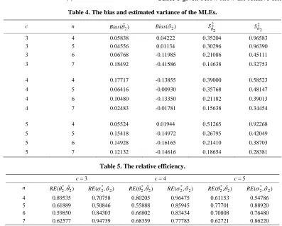
(3.11)Table 4 below displays the bias and the estimated variance of the MLEs of the location and scale parameters in this case.
2) When c is unknown: the maximum likelihood estimates of , and c can be obtained from (3.9) by solving the following three equations as
( )
1
( ) ( )
log log 0,
c
n
L i
i
L n L n
y n
c y y
(3.12)
1/
, c
L n
n y
(3.13)
11
1 0.
n L i
i L n
nc
c y
y
(3.14)4 Relative Efficiency
To compare between the BLUEs and the MLEs obtained in Sections 2 and 3, we calculate the relative efficiency in some cases as follows:
1) For the scale case we have RE( 1*, 1) = 1, 2) For the location-scale case we have
* *
* 2 * 2
2 2 2 2 2 2
ˆ ˆ2
2
( ) ( )
ˆ ˆ
( , ) =Var , ( , ) =Var .
RE and RE
S S
Table 5 given below show the relative efficiency
be-Table 4. The bias and estimated variance of the MLEs.
c n Bias(ˆ2)
2 ˆ ( )
Bias 2ˆ
2
S 2
ˆ2
S
3 4 0.05838 0.04222 0.35204 0.96583 3 5 0.04556 0.01134 0.30296 0.96390 3 6 0.06768 -0.11985 0.21086 0.45111
3 7 0.18492 -0.41586 0.14638 0.32753
4 4 0.17717 -0.13855 0.39000 0.58523
4 5 0.06416 -0.00930 0.35768 0.48147
4 6 0.10480 -0.13350 0.21182 0.39013
4 7 0.02483 -0.01781 0.15638 0.34454
5 4 0.05524 0.01944 0.51265 0.92268
5 5 0.15418 -0.14972 0.26795 0.42049
5 6 0.14928 -0.16165 0.21410 0.38703
5 7 0.12132 -0.14616 0.18654 0.28381
Table 5. The relative efficiency.
= 3
c = 4c = 5c
n *
2 ˆ2
( , )
RE RE( 2*,ˆ2) RE( 2*,ˆ2) RE( *2,ˆ2) RE( 2*,ˆ2) RE( *2,ˆ2)
[image:5.595.97.494.401.719.2]-tween the different estimates of the location and scale parameters. From Table 5, we see that, the BLUEs give more efficiency than the MLEs.
5. Acknowledgements
The author would like to thank the referees for their helpful comments, which improved the presentation of the paper. Also, the author would like to thank the Research Center, College of Science, King Saud University, for funding the project (Stat/2008/31).
6. References
[1] K. N. Chandler, “The Distribution and Frequency of Re-cord Values,” Journal of the Royal Statistical Society Se-ries B, Vol. 14, 1952, pp. 220-228.
[2] V. B. Nevzorov, “Records,” Theory of Probability and Its Applications, Vol. 32, 1988, pp. 201-228.
[3] H. N. Nagaraja, “Record Values and Related Statistics-A Review,” Communications in Statistics-Theory and Meth-ods, Vol. 17, 1988, pp. 2223-2238.
[4] M. Ahsanullah, “Introduction to Record Values,” Ginn Press, Needham Heights, Massachusetts, 1988.
[5] M. Ahsanullah, “Record values, The Exponential Distri-bution: Theory, Methods and Applications,” In: N. Balakrishnan and A.P. Basu Eds., Gordon and Breach Publishers, Newark, New Jersey, 1995.
[6] B. C. Arnold, N. Balakrishnan and H. N. Nagaraja, “A First Course in Order Statistics,” John Wiley & Sons, New York, 1992.
[7] B. C. Arnold, N. Balakrishnan and H. N. Nagaraja, “Re-cords,” John Wiley & Sons, New York, 1998. [8] N. Balakrishnan, M. Ahsanullah and P. S. Chan,
“Rela-tions for Single and Product Moments of Record Values from Gumbel Distribution,”Statistics & Probability Let-ters, Vol. 15, No. 3, 1992, pp. 223-227.
[9] N. Balakrishnan, P. S. Chan and M. Ahsanullah, “Recur-rence Relations for Moments of Record Values from Generalized Extreme Value Distribution,” Communica-tions in Statistics-Theory and Methods, Vol. 22, No. 5, 1993, pp. 1471-1482.
[10] N. Balakrishnan and M. Ahsanullah, “Relations for Sin-gle and Product Moments of Record Values from Expo-nential Distribution,” Journal of Applied Statistical Sci-ence, Vol. 2, 1995, pp. 73-87.
[11] N. Balakrishnan, M. Ahsanullah, and P. S. Chan, “On the Logistic Record Values and Associated Inference,” Journal of Applied Statistics, Vol. 2, pp. 233-248.
[12] K. S. Sultan and N. Balakrishnan, “Higher Order Mo-ments of Record Values from Rayleigh and Weibull Dis-tributions and Edgeworth Approximate Inference,” Jour-nal of Applied Statistical Science, Vol. 9, 1999, pp. 193-209.
[13] K. S. Sultan and M. E. Moshref, “Higher Order Moments of Record Values from Generalized Pareto Distribution and Associated Inference,” Metrika, Vol. 51, 2000, pp. 105- 116.
[14] A. A. Soliman, A. H. Abd Ellah and K. S. Sultan, “Com-parison of Estimates Using Record Statistics from Weibull Model: Bayesian and Non-Bayesian Ap-proaches,” Computational Statistics and Data Analysis, Vol. 51, No. 3, 2006, pp. 2065-2077.
[15] K. S. Sultan, “Higher Order Moments of Record Values from the Inverse Weibull Lifetime Model and Edgeworth Approximate Inference,” International Journal of Reli-ability and Applications, Vol. 8, No. 1, 2007, pp. 1-16. [16] A. Drapella, “Complementary Weibull Distribution:
Un-known or Just Forgotten,” Quality and Reliability Engi-neering International, Vol. 9, 1993, pp. 383-385. [17] G. S. Mudholkar and G. D. Kollia, “Generalized Weibull
family: A Structural Analysis,” Communications in Sta-tistics-Theory and Methods, Vol. 23, 1994, pp. 1149- 1171.
[18] R. Jiag, D. N. P. Murthy and P. Ji, “Models Involving two Inverse Weibull Distributions,” Reliability Engi-neering and System Safety, Vol. 73, No. 1, 2001, pp. 73-81.
[19] R. Calabria and G. Pulcini, “On the Maximum Likelihood and Least-Squares Estimation in the Inverse Weibull Dis-tributions,” Statistica Applicata, Vol. 2, No. 1, 1990, pp. 53-66.
[20] M. Maswadah, “Conditional Confidence Interval Estima-tion for the Inverse Weibull DistribuEstima-tion Based on Cen-sored Generalized Order Statistics,” Journal of Statistical Computation Simulation, Vol. 73, No. 12, 2003, pp. 887- 898.
[21] D. N. P. Murthy, M. Xie and R. Jiang, “Weibull Models,” John Wiley & Sons, New York, 2004.
[22] E. M. Nigm and R. F. Khalil, “Record Values from In-verse Weibull Distribution and Associated Inference,” Bulletin of the Faculty of Science, 2006.
[23] N. Balakrishnan and A. C. Cohen, “Order Statistics and Inference: Estimation Methods,” Academic Press, San Diego, 1991.