A comparison of level set models in image segmentation

IET Research Journals

Submission for IET Image Processing

A Comparison of Level Set Models in Image

Segmentation

ISSN 1751-8644 doi: 0000000000 www.ietdl.org

Roushanak Rahmat

_{, David Harris-Birtill}

Abstract:Image segmentation is one of the most important tasks in modern imaging applications, which leads to shape recon-struction, volume estimation, object detection and classification. One of the most popular active segmentation models are level set models which are used extensively as an important category of modern image segmentation technique with many different available models to tackle different image applications. Level sets are designed to overcome the topology problems during the evolution of curves in their process of segmentation while the previous algorithms cannot deal with this problem effectively. As a result there is often considerable investigation into the performance of several level set models for a given segmentation problem. It would therefore be helpful to know the characteristics of a range of level set models before applying to a given segmentation problem. In this paper we review a range of level set models and their application to image segmentation work and explain in detail their properties for practical use.

1 Introduction

Image segmentation is the process of partitioning the image into meaningful regions. It is one of the most important tasks in mod-ern imaging for shape reconstruction, volume estimation, object detection and classification. Many different algorithms have been proposed to solve image segmentation problems. In some applica-tions such as medical image segmentation, highly precise models are needed where strong assumptions and anatomical prior are often imposed on the expected segmentation results. The methods based on statistical theory methods can fail in the presence of noise as the artificial parameters should be considered as well, while a lot of physical phenomenon can be described by partial differential equa-tions (PDEs). Those based on PDE, began with the Snake technique introduced by Kass in 1987 [1]. The snake model is based on mini-mization of an energy term to halt the growth of evolving contours at edges or boundaries. It locks into edges and lines by taking advan-tage of image forces. Another popular image segmentation method is the level set, introduced in 1988 by Osher-Sethian [2] to over-come the shortcomings of the Snake method such as its topological problem as well as accurate prior knowledge for their initialization. Since level set models are independent of prior knowledge, they are very robust segmentation models when there is no ground truth available. Level set methods are used extensively and have many different applications. As a result there is often considerable investi-gation into the performance of several level set methods for a given problem. It would therefore be helpful to know the characteristics of a range of level set methods before applying any to a given segmen-tation problem. Several review papers on level set segmensegmen-tation are available but each is focused on one area or specific aspect of imag-ing applications. Some of these topics are: Region-based algorithms (Cremers in 2005 [3], Jiang in 2012 [4]); medical imaging (Suri in 2001 [5], Elsa Angilini in 2005 [6]); inverse problems and optimal design (Burger and Osher in 2005 [7]); piecewise constant applica-tion (Tai and Chan in region based methods in 2004 [8]); deformable models in general (Montagnat in 2001 [9], Suri in 2002 [10]); and a short general review (Bhaidasna in 2013 [11], Vineetha in 2013 [12]).

As image segmentation is a growing area of research many dif-ferent robust segmentation methods have been developed. Difdif-ferent methods such as threshold methods, edge based methods, region

based methods, clustering based methods, watershed transforma-tion, PDE-based methods and neural network methods which can be equally good and, depending on the choice of user, can perform well in modifying them in different models for different applica-tions. This paper reviews a range of different level set models and their application to image segmentation work and explains in detail their properties for image segmentation use. The advantages and disadvantages of each model are discussed and their properties and limitations when dealing with different images are compared.

There are many different applications for using a level set method. Sometimes new level set models are proposed to work on different applications. A review on this topic could be useful especially in view of the use of level set methods to specific problems. For exam-ple, in [60], Osher reviews a wide variety of problems involving external physics such as compressible and incompressible (possi-bly reacting) flow, Stefan problems, kinetic crystal growth, epitaxial growth of thin films, vortex-dominated flows, and extensions to mul-tiphase motion, computer vision and image processing. Also, there are many novel implementation of level set in different applications of imaging, such as image registration in [61], inhomogeneous med-ical image segmentation in [62], image denoising [63] and deep learning [64].

2 Active Contours

the separability of the dependent variables in an equation. In another definition, an explicit movement of a curve is independent of other values for the same level), therefore a single equation is used to eval-uate new nodal variables for a single time step. An implicit solution contains information obtained from solving simultaneous equations for the full grid for each time step. This is computationally more demanding but allows for larger time steps and better stability [57].

Fig. 1: Movement of a. geometric vs. b. parametric contours.

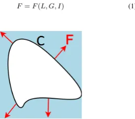
In Figure 2 the black boundary represents the contourCmoving with force/speed valueFand in the normal directionN perpendicu-lar to the interface, any tangential component will have no effect on the position of the front.Fdepends on local propertiesLsuch as cur-vature and normal direction, global propertiesGsuch as shape and position of the front and independent propertiesIthat do not depend on the shape of the front (some physical energies and properties such as heating on either side of the interface or fluid mechanical effects) [13, 14]. In general, the force or speed is the negative value of the energy field,F=−∇E. If the curve moves inward, then the speed value would be negativeF <0and if it moves outward, it would be positiveF >0.

F=F(L, G, I) (1)

Fig. 2: Contour evolution with speed value ofFin normal direction to the contourC.

Active contour model, also called snake is one of the first intro-duction to an explicit energy minimization contour. A snake model evolves a contour by dividing it into markers/points (parametris-ing the contour/gett(parametris-ing a number of samples of it). Its contourC is shaped based on tracking point positions in a Lagrangian frame-work that move with the value of the energy field (energy between the inside and outside of the contour).

Snake can be formulated by minimizing an energy functional con-sisting of an internal elastic energy termEinternalas well as an external edge-based energy termEexternalwhileCrepresents the 2D contour of segmentation asC(s) = (x(s), y(s)),s=0,..,1 which should be initialised first by the user close to the edges of interest:

ESnake=Einternal+Eexternal (2)

The internal energy defines the length of each contour which adjusts the deformations made to the snake. It controls the stiffness, rigidity and elasticity of the curve. The external energy helps in min-imizing the high-gradient areas in the image, it controls the contour to be better fitted onto the image. Equation 2 can be expanded into Equation 3, where the first two derivative terms refer to the internal energy and the final term represents the external energy.

ESnake=α

Z1

0|

C0|2ds+β

Z1

0|

C00|2ds+γ

Z1

0|∇ I(C)|2ds

(3) whereIrepresents the image inx−yplane,Crepresents the contour of segmentation,C0=dC

ds 2

the first derivative andC00= d2_C

ds2 2

the second derivative.αandβare a composition of the con-tinuity and the smoothness of the contour which are defined by the user.αwhich can control the continuity of the curve by defining the distance between sampling points in the curve. A larger value ofα can stretch the curve more.βcontrols the amount of curvature, a large value of it can lead to less oscillations in the contour.γis the weight of external energy or the edge functional which is based on the image gradient which is set to−1.

Snake model suffer from numerous shortcomings that the level set method overcomes [58]:

1. Dealing with topological changes: In situations where the curve merges with another curve or splits into two or more segments their performance is poor.

2. Self intersection and overlap: The explicit definition of a snake limits its re-gridding or re-parametrisation process and causes over-laps or self-intersection during the evolution.

3. Dependency on initialization: Their sensitivity to the first esti-mation of contour position and shape, which is because the non-convexity characteristic in the energy functional restricts further shape deformation.

4. Extension: Snake models are not able to be developed into other further segmentation applications using colour, texture or motion. 5. Sensitivity to noise: Snake performs weakly in a noisy gradi-ent field as its main formulation does not use region-based statistics whilst level set does.

3 Fundamentals of Level Set

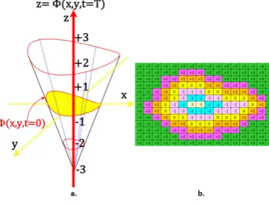
The level set was initially designed as an Eulerian formulation of a propagating front, which grows with the speedFperpendicular to the curve. Level set implicitly provides the propagation of the con-tour with good tracking of the topological changes. In other words, level set embeds a curve in 2D while growing in 3D, shown in Figure 3, where thezaxis represents values of functionφ(x, y, t) to match the evolution of the interface. The reason of having another dimension compared to snake is for better tracking of parametrisa-tion points that collide in snake. However, level set can stand at each point(x, y)and adjust the height of thezfunction which vanishes the topological problem. Such a level set is a growing or shrinking contour based on curvature-dependent speed for propagating fronts. It uses Hamilton-Jacobi equations to reconstruct complex shapes.

Fig. 3: Level set function in blue, and zero level set surface in yellow.

In this framework, at any timet, the frontΓ(t), implicitly defined by Equation 5, which shows that at each iteration, the new level set would be relocated at zero level again (called re-initialization). This is easily performed by recalculating the distance,z= 0, of every point from the contour, however it is computationally expensive.

Γ(t) ={(x, y)|φ(x, y, t= 0) = 0} (5) Figure 3 illustrates the formation of a level set function. It defines the propagating boundary/region as the zero level set,φ(x, y, t= 0), of a higher dimension on functionφ(x, y, t), wheretis time as the curve is evolving. The height (zaxis) corresponds to the min-imum distance from each point in a rectangular coordinate (image plane) from the contourC, based on the signed distancedfrom each point on(x, y)to the initial front, choosing a positive distance from outside the region and a negative direction from inside.

φ(x, t= 0)is required as the initial value (initialization) to start. Level set can be initialized automatically or semi-automatically in two or more phases depending on the decision of the user on how many different batches of segmentation are expected in an image. The two-phase level set method segments the image into two regions. Wherever three or four-phase level set methods exist, they can divide into three or four categories respectively by applying two separate level set functions at the same time. By considering only one level set function in 4.a. the yellow region represents the level set front at t= 0which is mapped to 4.b. on a contour on the 2D image. The inner parts of the contour represented with negative values which then decrease when they get farther from the zero level set and the outer points have positive value.

Fig. 4: Level set and its mapping in image plane.

In order for the points to always move/ride on the edge of the interface, level set should be re-initialised to zero level in each iteration of movement, Equation 6.

φ(x(t), y(t), t) = 0 (6)

Since the interface always corresponds to the place whereφ= 0, therefore outside of the edge dφ,t)

dt = 0. For better understanding this, consider tracking a particle~x= (x, y, z)on the surface in 3D over time:

dφ(~x, t)

dt = 0 (7)

from the chain rule, Figure 5 illustrates this:

Fig. 5: The chain rule demonstration of tracking a particle~x= (x, y, z)on the surface in 3D over time.

then,

dφ dt = 0−→

∂φ ∂x·

dx dt+

∂φ ∂y·

dy dt+

∂φ ∂z·

dz dt+

∂φ ∂t = 0 (8)

when, the directional derivative of a function∇f(x, y, z)is:

∇f=∂f dx~x+

∂f dy~y+

∂f

dz~z (9)

and the derivative of a vector~x= (x, y, z)is:

d~x dt=

dx dt+

dy dt+

dz

dt (10)

thus Equation 8 becomes:

∇φd~x+∂φ

dt = 0 (11)

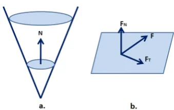
Since the signed distance of the level set at each point is required, therefore the surface normal at each point on the evolving front to its new position is necessary to be considered.d~x

dtis also known as the speed function_F~_{that defines the speed of the level set function and} how it evolves. It may also be written as_{F, while it comprised of the}~ normal and tangential components.

~

F=FNN~+FTT~ (12)

Fig. 6: Specifying the speed concept of level set method in the nor-mal and tangential direction in 3D space: a. level set in 3D and in its zero level: b. a surface in 2D.

thus, 11 may be written as:

∂φ

∂t +∇φ·F~= 0 (13)

which is a linear partial differential equation. Expanding 13:

∂φ

∂t +∇φ(FNN~+FTT~) = 0 (14) As stated in [15], the tangential component has no effect, it van-ishes into leading the scalar termFN to only specify the speed function in the normal direction. Equation 14 thus becomes:

∂φ

∂t+∇φVNN~= 0 (15)

also normal is the gradient scaled in unit length:

~ N= ∇φ

|∇φ| (16)

substituting Equation 15 into Equation 16:

∂φ ∂t +∇φFN

∇φ

|∇φ|= 0 (17)

∂φ ∂t +FN

∇φ2

|∇φ|= 0 (18)

replacing∂φ

∂t withφt, therefore:

φt+FN|∇φ|= 0 (19)

Re-initialization is repeated during evolution to prevent the occur-rence of sharp corners and prevent flatness by calculating newφ values depending on the specified speed function. Therefore each iteration grows already knowing the old level set and the penalty value defined.

φ(x, y, t+ 1) =φ(x, y, t) + ∆φ(x, y, t) (20) Osher-Sethian designed the motion based on magnitude of the gradient and mean curvature flow, which solves the level set geome-try problem as a PDE. Curvature plays the role of smoothing the level set to smooth the contours with the front symbolizing the boundary of the object when the propagation comes to a halt. The speed in the neighbourhood of the contour controls the motion of the front and should stop the propagation by tending towards zero at the limit of propagation. The speed is expressed as:

∂φ

∂t =|∇φ(x, y)|(ν+k(φ(x, y))) (21) whereν is a fixed parameter used to control the shrinkage or expansion andbalances the regularity, robustness of evolution and

k(φ(x, y))is the mean curvature of the level set function that stops leakage into small noisy parts. This can be calculated from:

k(φ(x, y)) =div(∇φ

|∇φ|) =

φxxφ2y−2φxφyφxy+φyyφ2x (φ2

x+φ2y)3/2

(22) whereφxandφyrepresent the first-order PDEs ofxandy respec-tively andφxxandφyydenote the second-order PDEs of each for the level set first functionφ(x, y). This model is the initial repre-sentation of the level set presented by Osher-Sethian, which exploits information from the curvature to increase the performance of the stopping point of the growing contours. Computation time as well as parameter setting and adjustment are the key limitations of this model.

The Key advantages of level set are [13, 58]:

1. The process can be fully-automatic or semi-automatic. 2. They do not need parametrisation of the contour. 3. They are less sensitive to noise than Snake. 4. They are easily extendible to higher dimensions.

5. Level set methods can easily segment sharp corners and change topological structure (topological flexibility) during propagation [13].

6. Good numerical stability.

The growth of a level set is simple and can be listed as follows:

1. Initialization of the level set by initializing the front. 2. Calculating the level set speed and growing model. 3. Iterate.

4. Matching the stopping criteria.

The differences between the various level set methods are mostly in the second step that will be explained and discussed in greater detail in the following sections.

3.1 Initialization

There are three main ways of initializing an active contour or level set:

1. Naive initialization. 2. Manual initialization. 3. Automatic initialization.

Naive initialization is when any random or simple geometric shape is chosen as the initial contour/boundary anywhere in the image. This method is easy and fast to initialize but it can result in lengthy convergence to the desired boundary and might take many iterations to calculate the proper segmentation. It can also converge to the wrong object in an image and lead to divergence. Manual ini-tialization would be when the user chooses to initialize the contour or interior point manually. This model can be time-consuming and dif-ficult for the user but is faster for propagation to reach the desired boundary. This model fails in high dimensional imagery because of the user’s limitation in visualizing these high dimensions. Auto-matic initialization can be performed in different ways, one major model is called centres of divergence (CoD) [16]. The other auto-mated methods are force field segmentation (FFS) [17] and poisson inverse gradient (PIG) initialization [18].

4 Different Level Set Methods

4.1 Osher-Sethian Model

Geodesic Active Contours- In this model, first introduced by

Caselles in 1997 [22], the level set stops at high-gradient locations by attenuating the speed, and the propagation is faster at smooth loca-tions. This is achieved by adding an addition term to Osher-Sethian’s model,g(|∇I|), which relates the speed term to the inverse of the gradient of the image. More formally:

∂φ

∂t =|∇φ|g(|∇I|)(div(

∇φ

|∇φ|) +ν) (23)

whereνis always positive and,

g(|∇I(x, y)|) = 1

1 +|∇Gσ(x, y)∗I(x, y)|2 (24) whereGσis a Gaussian convolution filter with standard deviation σ.

Shape Modelling with Front Propagation- Maladi, Sethian and

Vemuri in 1995, improved the early Osher-Sethian level set method by calculating the speed function based on the entropy-satisfying upwind finite difference and solving level set PDE function as a Hamilton-Jacobi type equation of motion [23]. In this model, the speed function’s stopping criteria is a fulfilment of Osher-Sethian’s method. In 2000, Leventon introduced a model based on a combi-nation of prior shape information and level set methods [24]. The deformable shapes as well as the probability distribution were pre-sented over the variances of a set of training shapes. At each iteration of the level set, an estimate is made based on prior shape information.

4.2 Snake-Based Level Set Methods

Li designed a new model based on Snake for solving the inho-mogeneity in intensity where an edge based level set model was developed based on gradient flow, which previous methods had dif-ficulty solving [27]. This model applies the energy minimization method, by minimizing the fitting energy in segmentation.

This energy is:

E(φ) =µP(φ) +λL(φ) +νA(φ) (25)

where,

P(φ) =

Z

Ω 1

2(|∇φ| −1)dxdy (26)

L(φ) =

Z

Ωg(I)δ(φ)|∇(φ)|dxdy (27)

A(φ) =

Z

Ω

g(I)H(−φ)dxdy (28)

and

g(I) = 1

1 +|∇Gσ_∗I|p, p≥1 (29) P(φ)is a penalty term in the energy functional that is used dur-ing evolution of level set. The stoppdur-ing operator,gis based on a Gaussian Kernel that forces the level set to converge to zero when approaching the edges.σis the standard deviation,Lrepresents the length of the contour with respect to the stopping operator ofgas its weight andAis the speed controller of the evolution which makes the contour to shrink if theνis positive and tends to expand when theνis negative.

The level set PDE function in this model is based on the Gateaux derivative which is:

∂φ(x, y) ∂t =−

∂E

∂φ (30)

This equation can be expanded further as:

∂E

∂φ = −µ(∆φ−div(

∇φ

|∇φ|)) −λδ(φ)div(g(I)∇

φ|∇φ|)

−νgδ(φ)

(31)

therefore,

∂φ

∂t = µ(∆φ−div(

∇φ

|∇φ|))

+λδ(φ)div(g(I)∇ φ|∇φ|) +νgδ(φ)

(32)

whereµis the penalizing coefficient,λis the coefficient for length andνrefers to the area. The ratio ofλandνdefines the stopping point of level set evolution because both of these terms contain edge information. The length term keeps the contour tight and the area helps the expansion of the contour.

Geodesic active contours, introduced by Kichenassamy [28] and

Caselles [22] are based on Snake. In these models, the speed function is calculated by applying minimal distance curves in a Riemannian space derived from the image. Given an image,I, and for a given differentiable curve,C(p), p∈[0,1], they define the energy as:

E(C) =

Z1

0

g(|∇I(C(p))|)|C0(p)|dp (33)

The PDE functional calculated via derivation of the Euler-Lagrange system is therefore:

∂C

∂t =g(|∇I|)κ ~N−(∇g(|∇I|). ~N)N~ (34)

Threshold Level Set, Taheri applied a threshold level set method

for brain tumour segmentation in 3D which does not depend on den-sity function estimation by using a global threshold for the speed function [29]. This semi-automatic model requires a user’s input to initialize the threshold value for the level set based on information from a region inside a tumour. For convex tumours, a spherical sur-face is chosen as the initial level set located in the middle of the tumour. For concave tumours several spheres are required due to the complexity of the shape. The threshold updates at every iteration during the evolution which should decrease as it gets closer to the boundaries while the contrast between tumour (foreground object) and non-tumour (background) is increasing. The threshold in this model can be calculated based on

Ti+1=µib −kσi, ib ≥0 (35)

b

µi=1 n

n

X

j=1

xij (36)

b

σi= 1 n−1

n

X

j=1

(xij−µi)b 2 (37)

∂φ(x, y, t)

∂t +F(x, y, t)k∇φ(x, y, t)k= 0 (38)

F=F0·F_I(i)−kφ (39) whereF0is the constant propagation determined by a positive number andFI(i)is based on image characteristics in the(i+ 1)th iteration. Propagation stops when a boundary is reached.kφis the smoothness parameter. The threshold level set specifies theFIfor each sample based on the diversity between the threshold values. Therefore, the larger diversity leads to faster propagation/speed.

FI(x, y, z) =i ∆ 2[

1 +sgn(∆) max(∆) −

1−sgn(∆) min(∆) ] (40)

where∆is equal toI(x, y, z)andsgnrepresents the sign function which defines whether the speed function ofFIiis inside or outside of the tumour and classed as positive or negative respectively for initializing the level set. This process tends to stop near the boundary of tumours when threshold variation becomes negligible.

4.3 Region-Based Level Set

Chan-Vese in 1990s improved Osher-Sethian’s model by consider-ing an energy minimization model instead of PDE, which permits automatic detection of interior contours [30, 31]. The imprvement of performance was dur to considering a piecewise constant and piece-wise smooth optimal approximations proposed by Mumford-Shah [32]. Mumford-Shah introduced an energy minimization method for segmentation [32]:

EM S(u, C) =

Z

Ω(u−u0) 2

dxdy+µ

Z

Ω\C|∇u| 2

dxdy+ν|C|

(41) Whereµandνare positive weight values,Cis the contour or closed subset inΩanduis an approximation of the imageu0in the optimal piecewise smooth shape. This model can be simplified by consideringuas the piecewise constant function ofciinside of each connectedΩi(Ω =SiΩi

S_{C) and}

ci=mean(u0)inΩ0.

E(u, C) =X i

Z

Ωi

(u0−ci)2dxdy+ν|C| (42) The problem of segmentation based on the Mumford-Shah model is that it is not easy to use due to the unknown value ofCand also the problem is not convex.

4.3.1 Two-Phase Chan-Vese without Edges: Chan-Vese developed their model to a two-phase level set method without edges that could segment the image into two regions, while performed robustly in the presence of noise. Their model had a great improve-ment over the older models while its simplification f the energy functional is applied based on the mean intensity values in each region of the level set (inside or outside in two-phase),c1andc2, which are defined as:

c1=

R

Ω(1_R−H(φ(x, y)))(I(x, y))dxdy Ω1−H(φ(x, y))dxdy

(43)

c2=

R

Ω(H(φ(x, y)))(I(x, y))dxdy_R ΩH(φ(x, y))dxdy

(44)

His the Heaviside function,

H(x) =

1 ifx≥0

0 otherwise (45)

At each iteration the values ofc1andc2change and must be recal-culated based on the level set of a new region to calculate a new speed function as:

F(c1, c2, φ) =

Z

Ω

(u0−c1)2H(φ)dxdy

+

Z

Ω(u0−c2) 2

(1−H(φ))dxdy

+

Z

Ω|∇ H(φ)|

(46)

The Chan-Vese level set evolution equation is as follow whereδ represents a one-dimensional Dirac function.

∂φ

∂t =δ(φ)[νdiv(

∇φ

|∇φ|)−(u0−c1)

2

+ (u0−c2)2)] (47)

One of the benefits of this model is that the initialization is based on characteristics of the region. However it is not stable for the inhomogeneous images and the necessary re-initialization makes it computationally expensive.

4.3.2 Vector-Valued Image Chan-Vese Method: In 2000 [31], Chan-Vese improved their model further into a vector-valued image which is widely used in different imaging applications such as texture analysis and colour imaging.

F(c+, c−, φ) = µ.L

+

Z

inside(C) 1 N

N

X

i=1

λ+i|u0,i−c+i|2dxdy

+

Z

outside(C) 1 N

N

X

i=1

λ−i|u0,i−c−i|2dxdy (48)

and the PDE is:

∂φ

∂t = δ[µ.div

∇φ

|∇φ|

−_N1

N

X

i=1

λ+i|u0,i−c + i|

2 dxdy

+ 1 N

N

X

i=1

λ−i|u0,i−c−i|2dxdy]

(49)

whereλ+andλ−are weighting parameters andc+i andc−i are the mean value ofithcomponent of the vector image inside and outside of the contours. The advantage of this model is its ability to converge on edges with or without significant gradient. [3, 34, 35].

F(c, φ) =

Z

Ω

(u0−c11)2H(φ1)H(φ2)dxdy

+

Z

Ω

(u0−c10)2H(φ1)(1−H(φ2))dxdy

+

Z

Ω(u0−c01) 2

(1−H(φ1))H(φ2)dxdy

+

Z

Ω

(u0−c00)2H(φ1)(1−H(φ2))dxdy

+

Z

Ω|∇H(φ1)| +

Z

Ω|∇ H(φ2)|

(50)

c11=mean(u0)∈ {(x, y) :φ1(t, x, y)>0, φ2(t, x, y)>0}

c10=mean(u0)∈ {(x, y) :φ1(t, x, y)>0, φ2(t, x, y)<0}

c01=mean(u0)∈ {(x, y) :φ1(t, x, y)<0, φ2(t, x, y)>0}

c00=mean(u0)∈ {(x, y) :φ1(t, x, y)<0, φ2(t, x, y)<0}

(51)

Therefore,

∂φ1

∂t = δ(φ1)[νdiv(

∇φ1

|∇φ1|)

−(u0−c11)2+ (u0−c01)2)H(φ2) +(u0−c10)2+ (u0−c00)2))(1−H(φ2))]

(52)

∂φ2

∂t = δ(φ2)[νdiv(

∇φ2

|∇φ2|)

−(u0−c11)2+ (u0−c01)2)H(φ1) +(u0−c10)2+ (u0−c00)2))(1−Hs(φ1))]

(53)

Fig. 7: Multi-phase level set and its mapping in image plane.

4.3.4 Other Chan-Vese Based Methods: A new parallel based level set model for the follow up radiotherapy image anal-ysis in [36] introduced a novel configuration of level set which was designed based on the concept of vector-valued imaging was introduced. The concept of a vector-valued image in level set is intro-duced first by applying the two-phase Chan-Vese method at the same time on different images, such as different RGB channels or differ-ent texture images, and averaging the force value in each image at each iteration as shown in Figure 8.

Fig. 8: Vector-valued Chan-Vese on RGB channels, [36].

In this model, the same image or feature is used while different level set models are applied for segmentation as it is illustrated in Figure 9 and Equations 54 to 57.

Fig. 9: Proposed parallel level sets in vector-valued image, [36].

Figure 9 demonstrates the possible parallel combination of the Chan-Vese and the Li models while any other models can be used. This combination helps to exploit the robustness of different models and let them to compensate each others errors by modifying the force of level set in each iteration by calculating the average forces of both methods.

FCV =

Z

Ω

(u0−c1)2H(φ)dxdy

+

Z

Ω

(u0−c2)2(1−H(φ))dxdy

+

Z

Ω|∇ H(φ)|

(54)

FLi=µP(φ) +λL(φ) +νA(φ) (55) Equation 54 and Equation 55 are the forces for Chan-Vese and Li level set models which are explained in Section 4.2 and 4.3.4 in more details.

F=1

2(FLi+FCV) (56)

φ(x, y, t+ 1) =φ(x, y, t) + ∆t.F (57) where∆tis the step size.

In 2011, Bara [55] used variational models for solving level set based on Mumford-Shah and level set methods. This model is independent to the digital image grids.

Zhang improved the Chan-Vese method by replacing magnitude of gradient instead of image intensity as the evolution term [37].

∂φ ∂t =δ(φ)(I

0₋u+v

2 ) (58)

later Zhang further improved this model and defined the energy function as [38]:

∂φ ∂t =

αδ(φ)(I0−u+v 2 ) max|I0₋u+v

2 |

(59)

This model is mainly designed for special surgery instruments in CT images for minimally invasive spinal surgery.

Zhang [39] proposed a local image fitting (LIF) model by consid-ering image local characteristics to improve the Chan-Vese method, more advanced than local binary fitting (LBF) introduced by Li [25]. To prevent re-initializations at each iteration, Zhang used a Gaussian smoother to regularize the level set function. In this work, the local fitted image fitting function is defined:

ILIF=m1H(φ) +m2(1−H(φ)) (60)

m1=mean(I∈(x∈Ω|φ(x)>0∩Wk(x))) (61)

m2=mean(I∈(x∈Ω|φ(x)<0∩Wk(x))) (62) whereWk(x)is the rectangular window filter, e.g., a constant window.

ELIF=1 2

Z

Ω|I(x)−I LIF

(x)|2dx, dx∈Ω (63) Also again in 2010, Zhang [53] developed a variational multi-phase level set for segmenting boundaries on MR images. The process of this model is to find the intensity values based on differ-ent Gaussian distributions which vary in means and variances, and transforms the result to other dimensions by using a sliding window to resist the overlap of different tissues. In the new domain, Zhang defined the maximum likelihood for each point, which unified in the whole domain to construct the variational level set evolution.

Liu [40] improved the Chan-Vese method by considering the local characteristic named local region-based Chan-Vese designed with a better effectiveness and robustness for inhomogeneous images. The Energy function is designed as:

ELBF(φ, f1(x), f2(2)) =

λ1

Z

Ω

Z

Ω

g(x−y)(I(y)−f1)2H(φ(y))dy dx

+λ2

Z

Ω

Z

Ω

g(x−y)(I(y)−f1)2H(φ(y))dy dx

+µ

Z

Ωδ(φ(x))|∇φ(x)|dx +ν

Z

Ω 1

2(|∇φ(x)| −1)dx

(64)

f1(x) =

R

Ωgk(x_R −y)(H(Φ(x, y)))(I(x, y))dxdy Ωgk(x−y)H(Φ(x, y))dxdy

(65)

f2(x) =

R

Ωgk(x_R −y)(1−H(Φ(x, y)))(I(x, y))dxdy Ωgk(x−y)(1−H(Φ(x, y))dxdy)

(66)

where f1(x) andf2(x) are the image approximate intensity means inside and outside the contourCandgrepresents the Gaus-sian Kernel filters.

Xiao-Feng Wanga [41] introduced a local Chan-Vese (LCV) consisting of three terms: global, local and regularizer. This new Chan-Vese model which formed based on the techniques of curve evolution, local statistical function and level set method performs a robust segmentation on images with intensity inhomogeneity.

ELCV= α·EG+β·EL+ER =α

Z

(inside(C))|

I−c1|2dxdy

+α

Z

(outside(C))|I−c2| 2

dxdy

+β

Z

(inside(C))|

gk∗I−I−d1|2dxdy

+β

Z

(outside(C))|gk∗I−I−d2| 2

dxdy (67)

whereEGis the global energy,ELis the Local,ERrepresents the regularizing term,gkis the averaging convolution operator and d1andd2are the approximate intensity means inside and outside of the contour with respect to the difference image,gk∗I−I.

Droskey in 2001, presented a multi-grid level set method for 3D medical image processing [45].By applying inter-active mod-ulation for the speed function this model can deal with non-sharp boundaries.

Ho in 2003, introduced a software package for level set by applying gradient based and region competition level set methods [46].

In 2008, Cheng [49] proposed a model based on the Chan-Vese level set method that uses shape prior knowledge for liver segmen-tation. A training set for prior shape is computed based on statistical models and in contrast to the previous shape prior of models this model allows the prior shape to be scaled, rotated or translated by applying an affine transformation.

In 1995, Kichenassamy and Tannenbaum in [28] modified ver-sion of snake on gradient flows relative to specific new feature-based Riemannian metrics. This model convergences based on the desired features that lie at the bottom of a potential well.

Lankton and Tannenbaum proposed a new robust region based segmentation model using level set which considers local rather than global statistical characteristics [42]. This model shows a great improvement in the case of inhomogeneous images.

E(φ) =

Z

Ωx δφ(x)

Z

Ωy

β(x, y).F(I(y), φ(y))dxdy

+λ

Z

Ωx

δ(φ(x))||∇φ(x)||dx

(68)

where,

β(x, y) =

1 if||x−y|| ≤r

0 otherwise (69)

therefore, ∂φ

∂t(x) = δφ(x)

Z

Ωy

β(x, y).∇φ(y)F(I(y), φ(y))dy

+λδφ(x)div(∇φ(x)

|∇φ(x)|)

The authors compared their model with three other region based level set methods and demonstrated an improvement with their algorithm, the other models compared were uniform modelling energy as introduced by Chan-Vese [30], the means separation energy by Yezzi and Tannenbaum [28] and the histogram separation energy by Michailovich and Tannenbaum [43].

Pereyra exploited information theory to define the Riemannian structure of the statistical manifold associated with the Chan-Vese active contour [44]. They used the Fisher information matrix to form the natural gradient metric of the statistical manifold which con-verges much faster than the Euclidean gradient descent algorithm. In this algorithm, log-likelihood for information geometry was defined as follows:

log(p(I;φ)) = −ΣNi=11₂(Ii−c1)2H(φi)

−ΣNi=11 2(Ii−c2)

2_H(

−φi)

−N₂log(2π)

(71)

The natural gradient matrix is defined as:

G(φ)(i,j)=|δ(φi)0 |(c1−c2)2if i=j and 0 otherwise (72)

whereδ0(x) =_π(−2_+x2x2₎2, therefore the re-initializer is based on:

φt+1=φt+ηtHG−1(φt)δ(φt)((Ii−c1)2−(Ii−c2)2) (73) where ηtis the time step at iterationtand H is the spatial smoothing operator of Hessian. For fast convergence, this model used the difference between energy functional of each iteration and the previous one.

In 2012, Yuan represented L2+Soblev gradient to improve Chan-Vese model for calculating the energy function which was computationally more efficient than its traditional models. This work presents theL2gradient for minimizing external energy and Soblev gradient for the internal energy which represents length of curve and produces the result in one iteration [56].

In 2003 Lefohn et al [47] introduced a new level set model based on interactive rates on commodity graphics cards (GPUs) for med-ical image segmentation. This model provides the user immediate feedback on the parameter settings and let the user to tune them separately in real time.

Lin [48] in 2004 prepared a new level set model based for medi-cal image segmentation on new speed function by considering the region intensity information, instead of the image gradient infor-mation. The proposed speed function governs the deformation of interface. Shi [50] introduced a fast two-cycle algorithm in 2008 for the approximation of level-set-based curve evolution which is suitable for real-time implementation.

In the same year, Cao [51] proposed a new energy functional used for variational level set approach for SAR images by consid-ering the statistical model of speckle noise in the energy functional. Accurately and automatically extracts the regions of interest in SAR images. Segmentation is based on minimization of the energy func-tional via level set which is suitable for SAR images due to their characteristics.

Also, Bernard [52] in 2009 introduced a continuous represen-tation of a level set based on B-Spline on medical images. The smoothness in this model can be explicitly controlled via the chosen B-spline kernel.

In 2010, El Hadji [54] made a variational and prior shape based level set in medical images by less reinitialization due to considering a penalization term that forces the level set to be close to a signed distance function (SDF). This model detects tumour boundaries in medical imaging while they are not homogeneous and it performs well in both prior and non prior shape based image segmentation.

5 Tuning Level Set Parameters

In general, the approach of variational or optimization problems is to assign a cost function to each element to see how this cost solves the problem, where a low score is a good match and a high score is a bad match. Once the cost function is designed, it should be noted that it can be difficult to find the global minima if the cost is not convex. Gradient descent or steepest descent methods work by initializing and then descending at each instance, the direction is checked by the derivative the slope or the curve. By respecting this rule and trying to keep the optimization equations always in a convex form, the param-eter setting in active contours and level set methods is simpler. By finding the most relevant parameters, the level set methods can be tuned to converge to appropriate boundaries. As previously pointed out, the lack of gold standard for lung/medical imaging makes find-ing the optimal parameters more challengfind-ing, requirfind-ing a greater depth of image analysis.

The parameter setting of each model defines a specific range for each parameter, therefore it is usually based on the model as well as the images used, each model presents different parameters for dif-ferent images. Some evolutionary algorithms applied with level set for better parameter settings are based on genetic algorithm [19], particle swarm optimization [20], or ant colony optimization [21].

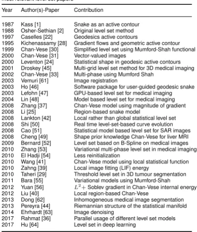
The Table 1 summarizes the history of the discussed papers and some other important papers using level set.

Table 1 A summary table showing a chronology of the key contribution of the most relevant level set papers

Year Author(s)-Paper Contribution

1987 Kass [1] Snake as an active contour 1988 Osher-Sethian [2] Original level set method 1997 Caselles [22] Geodesics active contours

1995 Kichenassamy [28] Gradient flows and geometric active contour 1999 Chan-Vese [30] Simplified level set using Mumford-Shah functional 2000 Chan-Vese [31] Vector-valued images

2000 Leventon [24] Statistical shape in geodesic active contours 2001 Droskey [45] Multi-grid level set method for 3D medical imaging 2002 Chan-Vese [33] Multi-phase using Mumford Shah

2003 Vemuri [61] Image registration

2003 Ho [46] Software package for user-guided geodesic snake 2003 Lefohn [47] GPU-based level set for medical imaging 2004 Lin [48] Model based level set for medical imaging 2008 Zhang [37] Chan-Vese model using magnitude of gradient 2008 Li [25] Region-based snake model

2008 Lankton [42] Local rather than global statistical level set 2008 Shi [50] Real time level-set-based curve evolution 2008 Cao [51] Statistical model based level set for SAR images 2008 Cheng [49] Shape prior knowledge Chan-Vese for liver MRI 2009 Bernard [52] Level set based on B-Spline on medical images 2010 Zhang [53] Variational multi-phase level set in medical imaging 2010 El Hadji [54] Less reinitialization

2010 Wang [41] Chan-Vese model using local statistical function 2010 Zahng [39] Local image fitting (LIF) energy

2010 Taheri [29] Threshold level set in 3D tumour segmentation 2011 Bara [55] Variational models using Mumford-Shah 2012 Yuan [56] L2_{+Soblev gradient in Chan-Vese internal energy} 2012 Liu [40] Local region-based Chan-Vese

2013 Dong [62] Inhomogeneous medical image segmentation 2013 Pereyra [44] Riemannian structure of the statistical manifold 2014 Ehrhardt [63] Image denoising

2017 Rahmat [36] Parallel usage of different level set models 2017 Hu [64] Level set in deep learning

6 Conclusion

7 References

1 Kass M, Witkin A, Terzopoulos D. Snakes: Active contour models. International journal of computer vision. 1988 Jan 1;1(4):321-31.

2 Osher S, Sethian JA. Fronts propagating with curvature-dependent speed: algo-rithms based on Hamilton-Jacobi formulations. Journal of computational physics. 1988 Nov 1;79(1):12-49.

3 Cremers D, Rousson M, Deriche R. A review of statistical approaches to level set segmentation: integrating color, texture, motion and shape. International journal of computer vision. 2007 Apr 1;72(2):195-215.

4 Jiang Y, Wang M, Xu H. A Survey for Region-based Level Set Image Segmen-tation. In Distributed Computing and Applications to Business, Engineering & Science (DCABES), 2012 11th International Symposium on 2012 Oct 19 (pp. 413-416). IEEE.

5 Suri JS, Liu K. Level set regularizers for shape recovery in medical images. In Computer-Based Medical Systems, 2001. CBMS 2001. Proceedings. 14th IEEE Symposium on 2001 (pp. 369-374). IEEE.

6 Angelini E, Jin Y, Laine A. State of the art of level set methods in segmentation and registration of medical imaging modalities. In Handbook of Biomedical Image Analysis 2005 (pp. 47-101). Springer, Boston, MA.

7 Burger M, Osher SJ. A survey on level set methods for inverse problems and opti-mal design. European journal of applied mathematics. 2005 Apr;16(2):263-301. 8 Tai XC, Chan TF. A survey on multiple level set methods with applications

for identifying piecewise constant functions. Int. J. Numer. Anal. Model. 2004 Jun;1(1):25-47.

9 Montagnat J, Delingette H, Ayache N. A review of deformable surfaces: topology, geometry and deformation. Image and vision computing. 2001 Dec 1;19(14):1023-40.

10 Suri JS, Liu K, Singh S, Laxminarayan SN, Zeng X, Reden L. Shape recovery algorithms using level sets in 2-D/3-D medical imagery: a state-of-the-art review. IEEE Transactions on information technology in biomedicine. 2002 Mar;6(1):8-28.

11 Bhaidasna ZC, Mehta S. A review on level set method for image segmentation. International Journal of Computer Applications. 2013 Jan 1;63(11). 12 Vineetha G, Darshan G. Level set method for image segmentation: a survey. IOSR

J. Comput. Eng. 2013;8:74-8.

13 Sethian JA. Level set methods and fast marching methods: evolving interfaces in computational geometry, fluid mechanics, computer vision, and materials science. Cambridge university press; 1999 Jun 13.

14 Dale AM, Fischl B, Sereno MI. Cortical surface-based analysis: I. Segmentation and surface reconstruction. Neuroimage. 1999 Feb 1;9(2):179-94.

15 Sethian JA, Smereka P. Level set methods for fluid interfaces. Annual review of fluid mechanics. 2003 Jan;35(1):341-72.

16 Xingfei G, Jie T. An automatic active contour model for multiple objects. In Pattern Recognition, 2002. Proceedings. 16th International Conference on 2002 (Vol. 2, pp. 881-884). IEEE.

17 Li C, Liu J, Fox MD. Segmentation of edge preserving gradient vector flow: an approach toward automatically initializing and splitting of snakes. In Com-puter Vision and Pattern Recognition, 2005. CVPR 2005. IEEE ComCom-puter Society Conference on 2005 Jun 20 (Vol. 1, pp. 162-167). IEEE.

18 Li B, Acton ST. Automatic active model initialization via Poisson inverse gradient. IEEE Transactions on Image Processing. 2008 Aug;17(8):1406-20. 19 Ghosh P, Mitchell M, Tanyi JA, Hung A. A genetic algorithm-based level

set curve evolution for prostate segmentation on pelvic CT and MRI images. Biomedical Image Analysis and Machine Learning Technologies: Applications and Techniques. 2009 Dec 31:127-49.

20 Ganta RR, Zaheeruddin S, Baddiri N, Rao RR. Particle Swarm Optimization clus-tering based Level Sets for image segmentation. In India Conference (INDICON), 2012 Annual IEEE 2012 Dec 7 (pp. 1053-1056). IEEE.

21 Jiang D, Xu B, Ge L. A Hybrid Multi-Cell Tracking Approach with Level Set Evolution and Ant Colony Optimization. In International Conference in Swarm Intelligence 2015 Jun 25 (pp. 213-221). Springer, Cham.

22 Caselles V, Kimmel R, Sapiro G. Geodesic active contours. International journal of computer vision. 1997 Feb 1;22(1):61-79.

23 Malladi R, Sethian JA, Vemuri BC. Shape modeling with front propagation: A level set approach. IEEE transactions on pattern analysis and machine intelligence. 1995 Feb;17(2):158-75.

24 Leventon ME, Grimson WE, Faugeras O. Statistical shape influence in geodesic active contours. In Computer vision and pattern recognition, 2000. Proceedings. IEEE conference on 2000 (Vol. 1, pp. 316-323). IEEE.

25 Li C, Kao CY, Gore JC, Ding Z. Minimization of region-scalable fitting energy for image segmentation. IEEE transactions on image processing. 2008 Oct;17(10):1940-9.

26 Zhang K, Song H, Zhang L. Active contours driven by local image fitting energy. Pattern recognition. 2010 Apr 1;43(4):1199-206.

27 Li C, Huang R, Ding Z, Gatenby JC, Metaxas DN, Gore JC. A level set method for image segmentation in the presence of intensity inhomogeneities with application to MRI. IEEE Transactions on Image Processing. 2011 Jul;20(7):2007-16. 28 Kichenassamy S, Kumar A, Olver P, Tannenbaum A, Yezzi A. Gradient flows and

geometric active contour models. In Computer vision, 1995. proceedings., fifth international conference on 1995 Jun 20 (pp. 810-815). IEEE.

29 Taheri S, Ong SH, Chong VF. Level-set segmentation of brain tumors using a threshold-based speed function. Image and Vision Computing. 2010 Jan 1;28(1):26-37.

30 Chan T, Vese L. An active contour model without edges. In International Con-ference on Scale-Space Theories in Computer Vision 1999 Sep 26 (pp. 141-151). Springer, Berlin, Heidelberg.

31 Chan TF, Sandberg BY, Vese LA. Active contours without edges for vector-valued images. Journal of Visual Communication and Image Representation. 2000 Jun

1;11(2):130-41.

32 Mumford D, Shah J. Optimal approximations by piecewise smooth functions and associated variational problems. Communications on pure and applied mathemat-ics. 1989 Jul 1;42(5):577-685.

33 Vese LA, Chan TF. A multiphase level set framework for image segmentation using the Mumford and Shah model. International journal of computer vision. 2002 Dec 1;50(3):271-93.

34 M. Rousson, Cue integration and front evolution in image segmentation, Ph.D. thesis, Nice (2004).

35 Lianantonakis M, Petillot YR. Sidescan sonar segmentation using active contours and level set methods. InOceans 2005-Europe 2005 Jun 20 (Vol. 1, pp. 719-724). IEEE.

36 Rahmat R, Nailon WH, Price A, Harris-Birtill D, McLaughlin S. New Level Set Model in Follow Up Radiotherapy Image Analysis. In Annual Conference on Medical Image Understanding and Analysis 2017 Jul 11 (pp. 273-284). Springer, Cham.

37 Zhang N, Zhang J, Shi R. An Improved Chan-Vese model for medical image seg-mentation. In Computer Science and Software Engineering, 2008 International Conference on 2008 Dec 12 (Vol. 1, pp. 864-867). IEEE.

38 Zhang K, Zhang L, Song H, Zhou W. Active contours with selective local or global segmentation: a new formulation and level set method. Image and Vision computing. 2010 Apr 1;28(4):668-76.

39 Zhang K, Song H, Zhang L. Active contours driven by local image fitting energy. Pattern recognition. 2010 Apr 1;43(4):1199-206.

40 Liu S, Peng Y. A local region-based Chanâ ˘A¸SVese model for image segmentation. Pattern Recognition. 2012 Jul 1;45(7):2769-79.

41 Wang XF, Huang DS, Xu H. An efficient local Chanâ ˘A¸SVese model for image segmentation. Pattern Recognition. 2010 Mar 1;43(3):603-18.

42 Lankton S, Tannenbaum A. Localizing region-based active contours. IEEE trans-actions on image processing. 2008 Nov;17(11):2029-39.

43 Michailovich O, Rathi Y, Tannenbaum A. Image segmentation using active con-tours driven by the Bhattacharyya gradient flow. IEEE Transactions on Image Processing. 2007 Nov;16(11):2787-801.

44 Pereyra M, Batatia H, McLaughlin S. Exploiting information geometry to improve the convergence properties of variational active contours. IEEE Journal of Selected Topics in Signal Processing. 2013 Aug;7(4):700-7.

45 Droske M, Meyer B, Rumpf M, Schaller C. An adaptive level set method for medical image segmentation. In Biennial International Conference on Informa-tion Processing in Medical Imaging 2001 Jun 18 (pp. 416-422). Springer, Berlin, Heidelberg.

46 Ho S, Cody H, Gerig G. Snap: A software package for user-guided geodesic snake segmentation. Submitted to MICCAI 2003. 2003 Apr.

47 Lefohn A, Cates J, Whitaker R. Interactive, GPU-based level sets for 3D segmen-tation. Medical Image Computing and Computer-Assisted Intervention-MICCAI 2003.

48 Lin P, Zheng CX, Yang Y. Model-based medical image segmentation: a level set approach. In Intelligent Control and Automation, 2004. WCICA 2004. Fifth World Congress on 2004 Jun 15 (Vol. 6, pp. 5541-5544). IEEE.

49 Cheng K, Gu L, Xu J. A novel shape prior based level set method for liver segmentation from MR images. In Information Technology and Applications in Biomedicine, 2008. ITAB 2008. International Conference on 2008 May 30 (pp. 144-147). IEEE.

50 Shi Y, Karl WC. A real-time algorithm for the approximation of level-set-based curve evolution. IEEE transactions on image processing. 2008 May;17(5):645-56. 51 Cao Z, Pi Y, Yang X, Xiong J. A variational level set SAR image segmentation approach based on statistical model. In Synthetic Aperture Radar (EUSAR), 2008 7th European Conference on 2008 Jun 2 (pp. 1-4). VDE.

52 Bernard O, Friboulet D, ThÃl’venaz P, Unser M. Variational B-spline level-set: a linear filtering approach for fast deformable model evolution. IEEE Transactions on Image Processing. 2009 Jun;18(6):1179-91.

53 Zhang K, Zhang L, Zhang S. A variational multiphase level set approach to simul-taneous segmentation and bias correction. In Image Processing (ICIP), 2010 17th IEEE International Conference on 2010 Sep 26 (pp. 4105-4108). IEEE. 54 Diop EH, Ba SO, Jerbi T, Burdin V. Variational and Shape Priorâ ˘A ˇRbased Level

Set Model for Image Segmentation. In AIP Conference Proceedings 2010 Sep 30 (Vol. 1281, No. 1, pp. 2139-2142). AIP.

55 Bara S, Kerroum MA, Hammouch A, Aboutajdine D. Variational image segmen-tation models: application to medical images MRI. In Multimedia Computing and Systems (ICMCS), 2011 International Conference on 2011 Apr 7 (pp. 1-4). IEEE. 56 Yuan Y, He C. Variational level set methods for image segmentation based on both L2 and Sobolev gradients. Nonlinear Analysis: Real World Applications. 2012 Apr 1;13(2):959-66.

57 Osher S, Fedkiw R. Implicit Functions. In Level Set Methods and Dynamic Implicit Surfaces 2003 (pp. 3-16). Springer, New York, NY.

58 Siddiqi MH, Lee S, Lee YK. Object segmentation by comparison of active contour snake and level set in biomedical applications. In Bioinformatics and Biomedicine (BIBM), 2011 IEEE International Conference on 2011 Nov 12 (pp. 414-417). IEEE.

59 Sussman M, Smereka P, Osher S. A level set approach for computing solutions to incompressible two-phase flow. Journal of Computational physics. 1994 Sep 1;114(1):146-59.

60 Osher S, Fedkiw RP. Level set methods: an overview and some recent results. Journal of Computational physics. 2001 May 20;169(2):463-502.

61 Vemuri BC, Ye J, Chen Y, Leonard CM. Image registration via level-set motion: Applications to atlas-based segmentation. Medical image analysis. 2003 Mar 1;7(1):1-20.

63 Ehrhardt MJ, Arridge SR. Vector-valued image processing by parallel level sets. IEEE Transactions on Image Processing. 2014 Jan;23(1):9-18.