Abstract—In this paper, a cost-effective and highly accurate resolver-to-digital conversion (RDC) method is presented. The core of the idea is to apply a third-order rational fraction polynomial approximation (TRFPA) for the conversion of sinusoidal signals into the pseudo linear signals, which are extended to the range 0-360° in four quadrants. Then, the polynomial least squares method (PLSM) is used to achieve compensation to acquire the final angles. The presented method shows better performance in terms of accuracy and rapidity compared with the commercial available techniques in simulation results. This paper describes the implementation details of the proposed method and the way to incorporate it in digital signal processor (DSP) based permanent magnet synchronous motor (PMSM) drive system. Experimental tests under different conditions are carried out to verify the effectiveness for the proposed method. The obtained maximum error is about 0.0014° over 0-360°, which can usually be ignored in most industrial applications.
Index Terms—Arc tangent function, Analog processing circuits, Pseudo linear signals, Resolver-to-digital conversion (RDC), Third-order rational fraction polynomial approximation (TRFPA).
I. INTRODUCTION
esolvers are extensively used as speed and angle measurement sensors in a variety of fields, including electric drive system and industrial servo system, because of their reliability, high efficiency and vibration-proof characteristics. Normally, the input of a resolver is excited by
high frequency signals. The output signals of a resolver contain angular position information, which is modulated by the high-frequency signals with sine and cosine waves.
The next step is to demodulate the resolver output signals and determine the angles. In many applications, an integrated circuit (IC), called resolver-to-digital converter (RDC), is used to extract the rotor position from resolver output signals.This is often used in industrial products, with the drawback of increasing the cost (about 25$ for 16bit resolver single chip AD2S1210, according to Digikey), which represents almost the 50% of a resolver cost (e.g., Resolver Tamagawa, 53$). Therefore, many software and hardware strategies have been proposed in literature [1]-[24] to realize RDC method with low cost hardware to achieve higher angle precision and faster responses, which can be mainly divided into open-loop and closed-loop methods.
Some open-loop methods are illustrated in [1]-[13]. For example, in [1]-[4], direct or indirect arc tangent computation is used with LUT stored in the EPROM or other storage. However, because of the functions nonlinearity, large amounts of data storage or even extra memory are needed. Limited sampling points and interpolation methods are the key issues. CORDIC (Coordinate Rotation Digital Computer) algorithm is another method suitable for fast calculation of trigonometric functions, mentioned in [5]-[7]. The only operations it requires are addition, subtraction, shift and a LUT. However, the accuracy of CORDIC algorithm is mainly affected by the limited number of iterations for microcontroller. Several other open loop methods are proposed to construct pseudo linear signals, described in [8]–[13]. Pseudo linear signals utilize the local nonlinear approximation of sine signals, cosine signals or their combination as linear signals and make a compensation for further linearization. In [8]-[10], the pseudo linear signals are made up of the difference between the absolute values of sine and cosine signals. In [11], a pseudo linear signal is obtained through appropriate mathematical manipulation between the auxiliary sinusoidal signals generated by plus and minus operation and the demodulated ones. In [12], multiple phase-shifted sinusoids (PSS) construct the pseudo-linear segments to determine the angle. The method proposed in [13] is based on computing a number of phase-shifted sine and cosine signals to reduce nonlinearity of the resulting tangent. For all the above mentioned open-loop methods, they utilize the different combination or operation from sine and cosine signals
A Resolver-to-Digital Conversion Method
Based on Third-order Rational Fraction
Polynomial Approximation for PMSM Control
Shuo Wang
1,2,
Student Member
, Jinsong Kang
1, Michele Degano
2,3, Member and
Giampaolo Buticchi
3,
Senior Member
Manuscript received June 09, 2018; revised October 07, 2018; accepted November 13, 2018. This work was supported in part by National Key Research and Development Program of China under Grant 2016YFB0100700 and in part by the Fundamental Research Funds for the Central Universities in China under Grant 1700219142 (Corresponding author: Shuo Wang).
S. Wang and J. Kang are with the College of Electronic and Information Engineering, Tongji University, Shanghai 201804, China (e-mail:[email protected];[email protected]).
S. Wang and M. Degano are with the Power Electronics, Machines and Control Group (PEMC Group), the University of Nottingham, Nottingham NG7 2RD, UK (e-mail:[email protected]). M. Degano and G. Buticchi are with the PEMC Group the University of Nottingham Ningbo China, Ningbo 315100, China (e-mail: [email protected]).
to construct pseudo linear signals, so there is no need to consider the stability and rapidity of RDC. However, such methods still need to compensate pseudo linear signals, either from the software part or from the hardware part. The accuracy for the angles has still a good margin of improvement.
Most of closed-loop methods employ commercially available the phase-locked loop (PLL), also called angular tracking observer (ATO) to achieve RDC as mentioned in [14]-[24]. Typical software implementations and hardware implementations are discussed in [14]-[21] and [22]-[24], respectively. The excitation signals and trigger signals for the ADCs are usually generated by a single microprocessor in [15]-[17] or high frequency wave generating chip in [22][23]. The resolver outputs are synchronously sampled and demodulated to enter two ADC channels for microprocessor. The final angle is obtained from demodulated sine and cosine signals using ATO algorithm. A typical ATO mentioned in [14]-[17] consists of a PI controller, an integrator, two trigonometric functions and four multiplications. In [18]-[19], the accuracy and time-delays issues for ATO are fully investigated. Double synchronous rotation coordinate system approach (DSRF) and Least Squares Method (LMS) are discussed in [20] and [21] aiming to improve the accuracy of angle measurement. In [20], oversampling methods and down-sampling finite-impulse response digital filters are introduced to reduce the time lag problems for ATO. Although the closed-loop ATO method has good noise immunity, delay, bandwidth and stability are still the key issues that many researchers are trying to address.
In this paper, a cost-effective and highly accurate open-loop method is proposed to realize RDC with a practical hardware and real-time software. Unlike other open loop methods, the absolute value of demodulated sine signals and cosine signals are transformed into pseudo linear signals directly by TRFPA method. The pseudo linear signals are then extended to 0-360° by means of the quadrants information. PLSM is used to compensate the angle error. Compared with common used methods and commercial solutions, the proposed method improves the accuracy of angle a lot and the cost of the system is reduced.
In Section II, the principle of the brushless resolver operation principle is described. The proposed approach is explained in Section III. Some simulation and experimental results are presented in Section IV and Section V, respectively. Section VI concludes this paper highlighting the outcomes.
II.BRUSHLESS RESOLVER PRINCIPLE
Fig.1. Electrical structure of a resolver
A typical structure of resolver is composed of one primary winding and two secondary windings, as shown in Fig.1. The resolvers operate like a special transformer excited by high frequency voltage in the primary windings. Generally, typical 1-15 kHz sinusoidal signals are applied on the primary winding as excitation signals, which introduce (1):
·sin(
t)
exc exc
V
E
(1)Where E is the amplitude of the excitation voltage, ωext is the
angular frequency of the excitation signals. Since the frequency of the exited signals is much higher than the electrical angular frequency of the motor, in practice, the condition is usually satisfied because of their relatively high frequency (typically a few kHz). The two secondary windings generate the following outputs signals:
e_ sin e_ cos
· ·sin( t) sin
· ·sin( t) cos
exc e
exc e
V k E
V k E
(2)
Where k is the transformation ratio and θe is the electrical angles of the motor. The equation (2) shows that the angles are modulated in sine and cosine signals with the high frequency excitation signals acting as carriers. Therefore, the resolver output signals require a suitable demodulation method to remove the carriers. In practice, one simple method mentioned in [15]-[17] is to trigger the sampling of analog-to-digital converter (ADC) when the excitation signal reaches its positive peak, which is a commonly applied technique. After demodulation, the signals become:
sin cos
· ·sin · ·cos
e
e
V k E
V k E
(3)
The most common and commercially applied method to determine θe is to utilize a four-quadrant arc tangent function:
sin
arctan( ) [0, )
cos 2
sin
-arctan( ) ( , ]
cos 2
sin 3
+ arctan( ) ( , )
cos 2
sin 3
2 -arctan( ) ( , 2 ]
cos 2
3
(sin 0,cos 0) (sin 0,cos 0)
2 2
e
e e
e e e
e
e e
e
e e e
e e e e
,
(4)
However, despite of its simplicity and feasibility, there are still some drawbacks as listed below:
1) The slope is quite high at zero-crossing point, which can lead to inaccuracies due to small interferences. When the cosine signals are approaching to the value zero, the result of the whole division is infinite, which may be unacceptable in the processor.
2) The equation (4) shows that the angle is not a continuous function. Because of the periodic nature of the arc tangent function, the full range of 360° is divided into four sections. For this reason, extra information is required to identify the sections.
1 S
2
S 1 C
2 C
1 E
2 E
Exci
tat
ion
winding
Cosine windi
ng
Sine winding
3) Direct arc tangent function can be difficult to use. In practice, the LUT method is commonly used to replace this function in [1]-[4]. However, the selecting sampling points and interpolation methods are limited by the sampling time. The more is the approximation detail, the larger is the resource occupied in the controller.
III.PROPOSEDCONVERSIONSTRATEGY
The basic principle of the proposed conversion strategy is depicted in the Fig.2. In Part I, the resolver output signals are demodulated. In Part II, the absolute values of the two signals are determined and the TRFPA method is used to make a conversion from sine and cosine wave into pseudo linear signals. In Part III, the final angles measurement is extended to the entire cycle and the quadrant of the angle is determined by the sign of the sine and cosine signals. In Part IV, PLSM method is utilized to make a compensation to acquire the final angles.
Fig.2. Block diagram of the proposed resolver conversion scheme
A.Third-Order Rational Fraction Polynomial
Approximation
The TRFPA method illustrated in [25] is used to replace the arc tangent function for theoretical analysis in image signals processing. In this paper, some basic theories have been revised so that they can be applied to practical RDC systems. The third-Order rational fraction polynomial approximation (TRFPA) is chosen, because of a tradeoff between the computational complexity and accuracy.
Due to odd function and periodic function features of arc tangent function, only the value in the first quadrant in [0, π/2] need to be taken into consideration for the angle. Then the proposed approximation method TRFPA can be written as (5). Note that the approximate result is normalized in the interval [0, 1] and the multiplication by π/2 can be done later, if necessary.
2 3
3 0 1 2 3
3 2 3
3 0 1 2 3
N ( )
( )=
( )
u
a
a u a u
a u
u
D u
b b u b u
b u
(5)
Where u equals to y/x, x and y stands for the sampling value of cosine and sine signals in the current time (x=cos
e, y=sin
e), respectively. The variables x and y are not independent and they have an intrinsic relevance (the square root of x2+y2 is unitary). The eight parameters a0a1 a2 a3 b0b1 b2 b3 are the coefficients required to be determined. The arctangent functionwith the following three properties enable the calculation of the
ai, bj (i,j=0,1,2,3) coefficients in a much simpler way: 3
arctan(0) 0 (0) 0 (6)
3
lim 2arctan( ) / 1 lim ( ) 1
x u
u u (7)3 3
0
1 2 1
arctan( ) arctan( ) ( ) ( ) 1
0 2
u
u u
u u u
(8)
These three constraints (6)(7)(8) are applied to (5) and (5) can be simplified as:
2 1 3 2 1
(u)
1
1
a u u
u
u
a u u
(9)The equation (9) is flexible, which can be transformed in polar coordinates with u=y/x.
Since only one coefficient a1 is required, this can be determined using the error function e3 (10) and the objective function J3 (11), defined as:
2 1
3 1 2
1 2
( , ) arctan( )
1 1
a u u u
e u a u
u a u u
(10)
1
2 1
3 0 2
1
2
min(max
arctan( )
)
1
1
a u
a u u
u
J
u
u
a u u
(11)Solving (11), the value of the parameter a1≈0.64039 is univocal, which corresponds to a maximum angle approximation error of about 0.00810°, which means that the RDC is up to about 15bit resolution (360°/32768) in the first quadrant. The derivation process and 3D-figure of the error are described in detail in the appendix. Substituting a1=0.64039 into (10) introduces:
2
3 2
0.64039 2
( ) arc
0.6403 tan( )
1 9
1
u u u
e u u
u u u
(12)
Substituting u= y/x into (12), the equation can be rewritten as a homogeneous formula:
2 2
3
3 2 2
3
0.6403 N ( , )
( , )= ( 0, 0)
( ,
9 0.64039 )
x y y x xy y
x y x y
D x y x y x xy y
(13)
Note that it is necessary to calculate the absolute values of sine and cosine signals before using (13), since the prerequisites are x>0 and y>0. Furthermore, when the cosine signals are approaching the value zero, the case of zero denominators for y/x is avoided.
Fig.3. Angle rearrangement for Part III
2 1 1 4 Case selector Case 1: Case 2: Case 3: Case 4: 4 2 2 ˆe 1 4 Case 1—4
3 E
sine
cose
1
0 0
1
0 0
11 Bit1Bit1 Bit0
TABLEI
QUADRANTS AND FINAL ANGLES Quadrant Bit1,Bit0 ˆe
I (0,0) 0.25×Eψ3
II (1,0) 0.5-0.25×Eψ3
III (1,1) 0.5+0.25×Eψ3
IV (0,1) 1-0.25×Eψ3
After the acquisition of the pseudo linear signals Eψ3, the sign of sine and cosine signals are acquired to determine the partition information, as shown in Fig.3. Considering the parity and periodicity of the functions, the entire range 360° for angles are divided into four quadrants in order to make full use of Eψ3's linear approximation. The relationship for the quadrant information and the pseudo-linear angle Eψ3 per unit is depicted in Table I. The logical operation Bit1 and Bit0 are calculated according to the sign of x and y, respectively. For example, when the sine wave is positive (Bit0=0) and the cosine is negative (Bit1=1), the angle estimation ˆ
e
is 0.5- 0.25Eψ3 per unit.
B.Angular Position Compensation Method
Fig.4. PLSM compensation method for error for Part IV
Applying x= cosθe and y= sinθe to (12) for the angle in [0,
π/2], the error e3 can be rewritten in polar coordinates:
2 2
3
0.6403
sin 9cos sin cos sin
2 ( )
sin cos 1 0.64039sin cos
e e e e e
e e
e e e e
e
(14)
Fig.4 describes the error e3 with black solid line. Seen from the figure, the error curves fluctuate in the period of 0-90° with six poles. The most popular methods used for curve fitting is the PLSM. Because of six poles in the range 0-90° (explained in appendix), a seventh order polynomial is selected and the polynomial coefficients are acquired by MATLAB simulation, described in (15). After the compensation by (15), the new error
̃ and the final angles ̃ can be written in (16) and (17), respectively.
6 5
3
4
3 7
2
ˆ ˆ ˆ ˆ
ˆ ( 20.2404 111.2857 239.6213 254.4939
ˆ ˆ ˆ
137.1434 33.9851 2.7004 0.0155) /1000;
e e e e
e e e
e
(15)
̃ ̂ (16)
̃ ̂ ̂ (17)
PLSM is used to reconstruct the error eˆ3 as shown in Fig.4, marked with dashed lines. The error shows quite perfect match with the true error e3 in (14). The curve of the new error e3 ( ̃ ̂ ) is marked with dotted lines. After compensation, the maximum error is reduced from 0.00810 ° to 0.0014°.
C. Simulation Process For Angular Position
Determination
Fig.5. Simulation of the angular position determination (a) the sine and cosine signals after demodulation (b) the sine and cosine signals after absolute value operation (c) pseudo linear signal after proposed approximation method (d) angular position before compensation (e) error before compensation (f) final angular position (g) new error after compensation
Fig.5 shows the results for angular position determination in the acceleration process. Fig.5(a) depicts the simulation results for the demodulated signals of two resolver output signals, which is converted into the absolute values in Fig.5 (b). The TRFPA is used to convert the two positive sine and cosine wave to pseudo linear signals Eψ3 shown in Fig.5(c). The
partition information related to the sign of sine and cosine signals can be used to extend Eψ3 to 0-360 degrees to acquire
the anglesˆe, as shown in Fig.5(d). The errors before and after compensation are shown in the Fig.5(e) and Fig.5(g), respectively. The final angles ̃ after complements are obtained finally, as shown in Fig.5(f). After compensation by means of PLSM, the maximum error is reduced from 0.0081° to 0.0014°.
IV.SIMULATION
Simulations results are shown in Fig.6 to make a precision comparison between the proposed method and two common methods arctangent LUT method and CORDIC method in the acceleration process. In our simulation tests, the LUT method is calculated by a finite number of values and improved by linear interpolation method, considering the storage space and sampling time constraints. The LUT is set according to the input signals values: 300 sampling points are selected in the range from -15 to 15; 85 sampling points are selected in the range from -100 to -15 and from 15 to 100; 18 sampling points are selected from the range of from -1000 to -100 and from 100 to 1000. The Maximum error values are 0.042 degrees depicted in the simulation results in Fig.6. Another method, based on CORDIC algorithm, takes 12 times iteration to complete the decoding angles for fast calculation of arc tangent function, described in [5]-[7]. Therefore, the maximum error values are 0.028°, which is about arc tan (1/211), as shown in Fig.6.
method shows only 0.0014°error in 17 bit resolution and the accuracy of the proposed method is greatly improved.
Fig.6 Simulation results comparing the errors using (a) arctangent LUT method, (b) CORDIC method and (c) the proposed method
The second simulation compares the proposed method with commercially available ATO method, when dealing with reference jumps, as shown in Fig.7. The parameters of PI controller for ATO method are designed according to [15][16]. The sample time Ts is the same as PWM period 100us. The reference angle jumps from 0° to 22.5° at 4Ts, from 22.5° to 45° at 8Ts and from 45° to 67.5° at 12Ts. Note that the simulation results are exaggerated in the actual process in order to test the response speed of the entire control loop. At these three time instants, the presented strategy shows good rapidity without any delay, while settle time (2Ts) or some overshoots (1.72°) exist in the result of the commercially available ATO scheme.
Fig.7 Simulation for proposed method compared with ATO method dealing with reference angle step
One more simulation for comparison between a commercially available ATO method and proposed method is shown with random noise superposed at the demodulated sine wave and cosine wave, as shown in Fig.8. In fact, input signals are always affected by interference or noise, such as the circuit system errors, AD sampling errors or sample/holder errors and so on. The motor is running at the speed of 150 rpm at the steady state. Then the Gaussian noise is added to the demodulated sine and cosine waves at 0.2s. The maximum
value of random noise is 10% of the sine amplitude, while the frequency is the same as the switching frequency 10 kHz, which is more serious than the actual experiment. At 0.3s, the motor is ramping with speed transients and finally settle down at 0.7s at the speed of 750 rpm. Compared the angle and error shown in Fig.8(c) and Fig.8(d), the maximum angle error for standard ATO is about 0.2rad, while the proposed method is about 0.1rad with less distortion. The proposed RDC strategy can presents a good speed dynamics and noise immunity, while commercially available ATO method presents more delay error, spikes and distortion.
Fig.8 Simulation for proposed method compared with ATO method dealing with noise environment (a) speed (b) demodulation signals(c) final angle and error using proposed RDC(d) final angle and error using
standard ATO (e) zoom figure TABLEII
COMPARISON OF DIFFERENT RDC METHODS
Methods Accuracy Calculation burden Immunity Noise Rapidity
CORDIC (13 bit) 0.028° low medium fast
LUT (13 bit) 0.042° high low fast
TRFPA 0.0014° (17 bit) low high fast
ATO
0.0879° (12 bit for
RDC IC) high high
delay or overshoots
In conclusion, , Table II shows the results obtained with the proposed method in comparison with three commonly used industrial methods considering the following figures of merit: accuracy, calculation burden, noise immunity and delay problems. The TRFPA method shows highest accuracy about 17bit resolution (360°/21 7=0.0027) theoretically. The
calculation burden is lower compared with ATO and LUT,
-0.05 0
0.05 iaibic(A)
-0.02 0 0.02
0.02 0.03 0.04 0.05 0.06 0.07 0.08 0.09 0.1 -0.002
0
0.002
Arctangent LUT method
Proposed method CORDIC method
time(s)
error(°
)
error(°
)
error(°
)
0
37.5
75
angle(degree)
0
37.5
75
angle(degree)
0
4Ts
8Ts
12Ts
16Ts
Kp=220,Ki=50 Kp=200,Ki=50
22.5°
Kp=180,Ki=50 ATO method Proposed method
overshoots1.72°
delay
reference angle acquired angle
45°
67.5°
22.5°
45°
67.5°
-2 0 2
-2 0 2 4 6 8
0.8 0.84 0.88 -20
2 4 6 8 200
400 600 800
iaibic(A)
-2 0 2
-2 0 2 4 6 8
0 0.2 0.4 0.6 0.8 -2
0 2 4 6 8
speed(rpm)
Voltage(V)
angle(rad)
angle(rad)
Steady state I Steady state II
speed transients
150rpm
750rpm
Adding gaussian noise
Adding gaussian noise
angle
(a)
(b)
(c)
(d) Adding gaussian noise
angle error
error
Delay error
time(s)
(e1)
(e2)
(e3) (e4)
(e5)
(e1)
(e2)
(e3)
(e4)
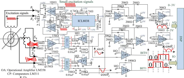
Fig.9. Detailed implementation of the proposed RDC
since both ATO and LUT need to store a large number of trigonometric functions and they need interpolation to compensate. As far as external noise immunity is concerned, ATO and TRFPA show good robustness compared with other two methods, however, undesired delays and overshoot problems occur for ATO method. The reason is that ATO method utilizes both current and last sampling points, and a PI controller and an integrator are used. Therefore, the stability is a key issue to be addressed while applying the ATO method. In summary, the TRFPA method shows better performance compared with other methods in terms of accuracy, calculation burden and rapidity.
V.IMPLEMENTATIONANDEXPERIMENT
Since the proposed RDC method is based on some basic operations, such as addition, multiplication, division andquadrant judgment operation, it can be implemented by all analog circuits to cut down the cost. In this particular work, a DSP28335 is used to implement the field-oriented control (FOC) algorithm for PMSM drive, the proposed RDC method can be completed by bespoke analog circuits and abovementioned DSP interfaces.
A. Converter Circuit
The detailed analog interface circuits for implementing the RDC are shown in Fig. 9. Most chips prices are given in Table III according to the Digikey or Farnell. The 10 kHz excitation signals are generated by a voltage controlled oscillator IC ICL8038 and then applied to the resolver by a push-pull power amplifier. The operational amplifiers OA3 and OA4 constitute two differential subtractors to acquire resolver output signals. Two sample-holders IC LF398 are utilized to demodulate the output signals, when the excitation signals reach their positive peak values by means of two comparators CP1 and CP2). The operational amplifiers OA5-OA8 achieve the absolute values of the signals transformation. The operational amplifiers OA9 and
OA10 are used to adjust the voltage to the range 0-3V which DSP can accept. The total cost of the whole circuit can be estimated at $6.12 in total, less than the commercial IC (RDC IC AU6802).
TABLEIII
PRICE COMPARISON BETWEEN PROPOSED METHOD AND COMMERCIAL METHODS
Proposed
Method Price
Commercial
Method Price
ICL8038 $0.66 AU6802 $18.5 LF398 $0.81×2 74LVC245AD $0.2×2 LM311 $0.21×4 Crystal Oscillator $0.12 LM358 $0.12×10 LM358 $0.12×2 Push-pull
Circuits $1.30
Push-pull
Circuits $1.30 Others $0.50 Others $0.50 Total $6.12 Total $21.06 Key points are:
1) The two differential amplifier circuits are used to reduce the common mode interference of the whole circuit. Other minor details are ignored, such as pull-up resistors and decoupling capacitors in the Fig.9, which are less significant to illustrate the converter functionalities. 2) The ICL8038 is used as a high frequency waveforms
generator, which can be replaced by an expensive Digital to Analog (DA) or PWM with low pass filters. For PWM method, synchronization could be an issue.
3) The absolute value circuits can be embedded in the DSP chip itself. However, the external absolute value circuits with the operational amplifiers OA5-OA10 are used to make full usage of the AD input range. Without the rectifier circuit, 1 bit of precision would be lost.
4) The comparators CP3 and CP4 are designed to reduce the zero-crossing error of the sine and cosine signals. The threshold for the change of the signal symbol is ±0.01, which is a negligible error for quadrant judgment. Without such threshold, quadrant misjudgment may occur for the final angle signals.
1 S 3 S 4 S 2 S 1 R 2 R Excitation signals Excitation signals 10kHz +15V -15V OA _ +
15k
15k
30k
30k
+15V
-15V
OA
_ +
15k
15k
30k
30k
LF398 LF398 +15V +15V -15V -15V 0.01uF 0.01uF
0.01uF 0.01uF 0.01uF 0.01uF
10k 10k
10k 10k 5V
CP+_ 5V
5V
CP_+ 5V
ICL8038 -15V OA _ + +15V -15V OA _ + +15V -15V OA _ + +15V
20k
20k
20k20k 20k
20k
10k
-15V OA _ + +15V -15V OA _ + +15V
20k
20k
20k20k 20k
20k
10k +15V -15V 0.1uF -15V OA _ + +15V
Small excitation signals
sine
| sin |
e| cos |
e-15V +15V +15V 10 k 10 k -15V -15V +15V 4.7k
10 k 10 k 10 k
1k
10k
2.7
4
k
100k
10k
4.7k
10k
+15V
10k
1k
1k
cos
e5V CP _+ 5V CP _+ 100k
1k
1k
BIT0 BIT1 AD IO DSP 1 2 3 4 5 6 8 7 1 2 3 4 OA: Operational Amplifier LM358
CP: Comparators LM311 R:1% +15V -15V OA _ +
30k
10k
10k 9 30k
+15V
-15V
OA
_ +
30k 10k
10k 10
30k
0~3V 0~3V
1
0
0
1
0
0
1
1
100k
10 k 1 3 2 4 56
7 8 1 3 2 4 56
5) Two RC circuits have been added to the signals of sine and cosine wave before the sample-holders LF398, in order to ensure that there is no spike at the sampling point. The RC time constant values for the filter have been chosen to less than 100μs, which can be compensated subsequently in the processor. Without such delay elements, there may be some spikes for the output signals after sample-holders.
B. Experimental Setup
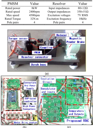
The PMSM test rig and its controller used for testing the proposed RDC is shown in Fig.10(a) and Fig.10(b). The detailed circuit for proposed RDC is shown in Fig.10(c). Seen from Fig.10(a), the platform consists of an 8kW 4-pole pairs PMSM incorporating a 5:1 reduction gear with a resolver (Tamagawa Type: J52XU9734A) installed as angle sensor. The detail parameters for PMSM and resolver are listed in Table IV. A processor DSP (Type: TMS320F28335) is the core component of the system to achieve both RDC and FOC algorithm. In order to show the better results of the intermediate process, the outcome transmits signals to four digital-to-analog converters (DAC) (Type: MAX538 with AMS1117-2.5 as reference voltage) with 12-bit resolution for the oscilloscope to display. A commercial PLL-type RDC special IC (Type: AU6802N1 with selectable resolution mode, 10Bit or 12Bit) is used for comparative tests.
TABLEIV
PMSM AND RESOLVER PARAMETERS
PMSM Value Resolver Value
Rated power 8kW Input impedances 80±12Ω Rated speed 2400rpm Output impedances 350±51Ω
Max speed 4500rpm Excitation voltages 7V RMS Rated Torque 32N.m Excitation frequency 10kHz
Pole pairs 4 Pole pairs 4
(a)
(b) (c)
Fig.10. Experimental test bench (a) PMSM test bench (b) Motor drive system (c) proposed RDC
C. Experimental Results
To verify the effectiveness of the proposed method, several experiments are carried out on PMSM drive system from low speed range to high speed range. Due to the restriction of the motor itself, the maximum speed can only reach 4500rpm. Note that it is hard to show all experimental waveforms under all conditions. Therefore, two typical speeds, 250rpm and 4250rpm are selected as low speed range representatives and as high speed range representatives, as shown in Fig.11 and Fig.12 respectively. In Fig.11, the pseudo linear signals Eψ3 are extended to a complete 0-360° range according to the partition information Bit0 and Bit1 (corresponding to Part III in Fig.3), and also the final angle waveforms after PLSM compensation are demonstrated. The corresponding pseudo linear signals, final angles signals and demodulated sine and cosine signals at the speed of 4250rpm are shown in Fig.12. By comparing all these signals shown in the oscilloscope with the simulation results in Fig.5, the obtained signals show perfect matches with the simulation results. The wide speed range and feasibility for the algorithm are confirmed.
Fig.11. The pseudo linear signals (Upper), final angle (Upper-middle) and the partition information bit0 and bit1(Lower) for the speed 250rpm
Fig. 12 The pseudo linear signals (Upper), final angle signals and the demodulation results for sine and cosine signals (Lower) for 4250rpm
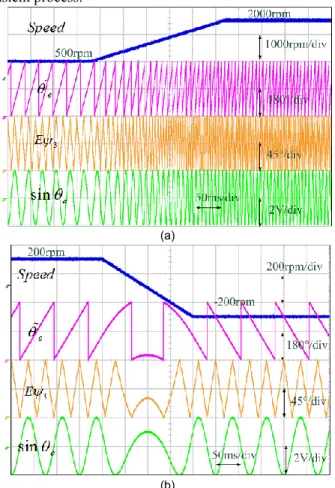
perfect ascending frequency tracking with the rising speed. The proposed RDC method shows perfect tracking property both in steady state and in the accelerating transient process. Another test results in Fig.13(b) shows the transient process, when the PMSM is running from positive 200rpm to reverse 200rpm. The pseudo linear signals Eψ3 and the final angles demonstrate descending and reversal frequency property with less distortion with variable direction operating conditions, which proves that the proposed method can be applied in both directions for transient process.
(a)
(b)
Fig. 13 The experimental results for speed (Upper), final angle (Upper middle), pseudo linear signals (Lower middle) and sine signals (Lower) dealing with (a) rising speed (b) descending and reversing speed
Fig.14. The error between the proposed method and accurate arc tangent signals: Standard angle (Upper) the angle acquired by proposed method (Upper-middle), the error without compensation
(Lower-middle), the error with compensation (Lower)
The last experimental test is conducted to assess the accuracy between the proposed methods and commercial RDC with standard high accurate arc tangent signals. The commercial RDC IC AU6802N1 is firstly tested. Seen from chip manual, two selectable resolution modes are commonly used for the commercial Chip, 10Bit for ±2LSB and 12Bit for ±4LSB. Note that the max error is 0.35° (360°×4/4096=0.35°) for 12bit mode and 0.70°(360°×2/1024=0.70°) for 10bit mode. In the actual measurement of AU6802N1, the maximum error is about ± 0.1° for 12bit mode, compared with high accurate arc tangent function.
The experimental results of accuracy comparison between the proposed method and high accurate arc tangent function are conducted at the speed of 600rpm depicted in Fig.14. Seen from Fig.14, the errors before and after compensation by PLSM are 18000 times the magnifications for DA output. The maximum angle error ̂ before compensation is less than ±0.01° and the maximum angle error ̃ after compensation is less than ±0.002° shown in the oscilloscope, quite matched with the theoretical values ±0.00810° and ±0.00140°. Under different speed conditions, the maximum experimental angle error is about 0.01°, quite higher with respect to the theoretical one, which can still be considered as negligible error in most industrial applications. Non-idealities in the ADC and in the operational amplifier can be recognized as the source of the error. A more accurate investigation on how the analog circuits affect the angle tracking will be object of future research.
VI.CONCLUSION
In this paper, it has been demonstrated how the proposed method provides a reliable, low-cost and high-precision solution for high speed and high performance motor position detection system. The new scheme utilizes the third-order rational fraction polynomials (TRFPA) to achieve approximations for precise triangular wave with two absolute values of sine and cosine signals. The pseudo linear signals are rearranged to the final angle signals compensated by PLSM method within the full range 0-360°. After compensation, the accuracy of angles is less than 0.00140° theoretically and less than 0.01° practically, which can be considered negligible in most high-precision industrial applications. A simulation comparison between different methods has been shown highlighting the benefits of the proposed method. For the implementation, only two ADC channels of a commercially available DSP and some common low-cost chips are needed. The proposed method is advantageous because of the low-cost, low computational effort and high accuracy, as demonstrated by the experimental verification.
APPENDIX
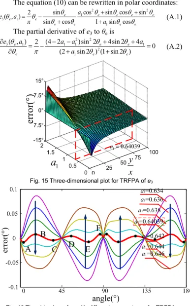
The minimum value of (A.1) is figured out under the condition that (A.2) is satisfied. Since the direct solving (A.2) may be a more complex calculation, some analytical methods such as Newton interpolation or particle swarm optimization are suitable for solving such problem. The optimal value for a1
0.00810°. The changing trend can be seen more clearly from the 3-D plot of e3 in Fig.15. The red dotted line frame represents the location optimal parameter a1. Fig. 16 depicts the side view of Fig. 14 with different parameter a1. The arrow indicates the direction of increase of a1. The bold red line is the optimal parameter a1 to be found. The optimal value for a1 is 0.64039 and the maximum angle approximation error is 0.00810°, which is a very slight error in practical application. Under the selected optimal parameter 0.64039, the error curves fluctuate in the period of 0-90° with six poles, from left to the right, listed as:A(3.438°,-0.0081°),B(16.616°,0.0078°),C(35.523°,-0.0041° ),D(54.431°,0.0041°),E(73.912°,-0.0078°), F(86.517°,0.0081°), which can be compensated by seventh-order PLSM method.
The equation (10) can be rewritten in polar coordinates:
2 2
1
3 1
1
sin cos sin cos sin
2 ( , )
sin cos 1 sin cos
e e e e e
e e
e e e e
a e a
a
(A.1)
The partial derivative of e3 to θe is
2 2
3 1 1 1 1
2 1
( , ) 2 (4 2 )sin 2 4sin 2 4
0
(2 sin 2 ) (1 sin 2 )
e e e
e e e
e a a a a
a
(A.2)
Fig. 15 Three-dimensional plot for TRFPA of e3
Fig. 16 The side view of e3 with different parameter a1 for TRFPA.
REFERENCES
[1] C. Attaianese and G. Tomasso “Position measurement in industrial drives by means of low-cost resolver-to-digital converter”, IEEE Trans. Instrum. Meas. vol. 56, no. 6, pp. 2155–2159, Dec. 2007.
[2] A. Khattab, M. Benammar and F. Bensaali “A Novel method for online correction of amplitude and phase imbalances in sinusoidal encoders signals”, Proc. Int. Power Electron. Motion Control Conf. (PEMC), pp. 784-789, Sep. 2016.
[3] S. Sarm, V.K. Agrawal and S. Udupa “Software-based resolver-to-digital conversion using a DSP”, IEEE Trans. Ind. Electron., vol. 55, no. 1, pp. 371-379, Jan. 2008.
[4] Shi, Tingna, Yajing Hao, and Guokai Jiang. “A method of resolver-to-digital conversion based on square wave excitation”, IEEE Trans. Ind. Electron. vol.65, no.9, pp. 7211-7219, Dec. 2018
[5] Ruifeng Y, Chenxia G, Peng Z. “The Method on Improving Digital Decoding Accuracy of the Resolver”, IEEE Sixth Int. Conf. on Instrum. Meas. Comp. Communi. and Contr.(IMCCC), pp. 745-751.May. 2016. [6] P. K. Meher, J. Valls, T.-B. Juang, K. Sridharan, and K. Maharatna, “50
years of CORDIC: Algorithms, architectures, and applications,” IEEE Trans. Circuits Syst. I, Reg. Papers, vol. 56, no. 9, pp. 1893–1907, Sep. 2009.
[7] Yepez, Juan, Xiaofeng Shi, and Seok-Bum Ko. “An FPGA-based Closed-loop Approach of Angular Displacement for a Resolver-to-Digital-Converter”. IEEE Int. Sym. on Circuits and Systems (ISCAS), May 2018.
[8] M. Benammar, L. Ben-Brahim, and M. A. Alhamadi, “A novel resolver to-360 linearized converter,” IEEE Sensors J., vol. 4, no. 1, pp. 96–101, Feb. 2004.
[9] M. Benammar, L. Ben-Brahim, and M. A. Alhamadi, “A high precision resolver-to-dc converter,” IEEE Trans. Instrum. Meas., vol. 54, no. 6, pp. 2289–2296, Dec. 2005.
[10] M. Benammar. “A novel amplitude-to-phase converter for sine/cosine position transducers”, Int. J. of Electron. vol. 94, no. 4, pp. 353-365, Apr. 2007.
[11] Y. Wang, Z. Zhu, and Z. Zuo, “A novel design method for resolver-to digital conversion”, IEEE Trans. Ind. Electron., vol. 62, no. 6, pp. 3724– 3731, Jun. 2015.
[12] M. Benammar, L. Ben-Brahim and M.A. Alhamadi. “A novel method for estimating the angle from analog co-sinusoidal quadrature signals”, Sensors and Actuators A: Physical, vol. 142, no. 1, pp. 225–231, Mar. 2008.
[13] A. Khattab, S. Saleh, M. Benammar and F. Bensaali “A precise converter for resolvers and sinusoidal encoders based on a novel ratiometric technique”, Proc. IEEE Sensors Appl. Symp. (SAS), pp. 100-105, Apr. 2016.
[14] Datlinger, Christoph, and Mario Hirz. “Investigations of Rotor Shaft Position Sensor Signal Processing in Electric Drive Train Systems.” 2018 IEEE Transport. Electrif. Conf. and Expo. (ITEC Asia-Pacific). Jun. 2018.
[15] D. A. Khaburi “Software-based resolver-to-digital converter for DSP-based drives using an improved angle-tracking observer” IEEE Trans. Instrum. Meas. vol. 61, no. 4, pp. 922-929, Apr. 2012.
[16] M. Caruso, A. O. Di Tommaso, F. Genduso, R. Miceli and G. R. Galluzzo. “A DSP-based resolver-to-digital converter for high-performance electrical drive applications,”. IEEE Trans. Ind. Electron. vol. 63, no. 7, pp. 4042-4051, Jul. 2016.
[17] N. Abou Qamar, C. J. Hatziadoniu and H. Wang “Speed error mitigation for a DSP-based resolver-to-digital converter using autotuning filters” IEEE Trans. Ind. Electron. vol. 62, no. 2, pp. 1134-1139, Feb. 2015. [18] Hanselman D C. “Resolver signal requirements for high accuracy
resolver-to-digital conversion”. IEEE Trans. Ind. Electron., vol.37, no.6, pp. 556-561. Dec.1990
[19] Lidozzi, A “Resolver-to-digital converter with synchronous demodulation for FPGA based low-latency control loops”.19th Euro. Conf. on Power Electron. and App. (ECCE Europe), Sept. 2017. [20] J. Bergas-Jané, C. Ferrater-Simón, G. Gross, R. Ramírez-Pisco, S.
Galceran-Arellano and J. Rull-Duran “High-accuracy all-digital resolver-to-digital conversion.”, IEEE Trans. Ind. Electron. vol. 59, no. 1, pp. 326-333, Jan. 2012.
[21] R. Hoseinnezhad, A. Bab-Hadiashar and P. Harding “Calibration of resolver sensors in electromechanical braking systems: A modified recursive weighted least-squares approach.”, IEEE Trans. Ind. Electron., vol. 54, no. 2, pp. 1052-1060, Apr. 2007.
[22] M. Benammar and A. S. P. Gonzales “Position measurement using sinusoidal encoders and all analog PLL converter with improved dynamic performance.”, IEEE Trans. Ind. Electron. vol. 63, no. 4, pp. 2414-2423, Apr. 2016.
0 25
50 75
100
0 0.5 1 1.5 2 -15° -7.5° 0° 7.5° 15°
1
a
y
x
1 0.64039
a
error(°
)
0 45 90 135 180
-0.1 -0.05 0 0.05
0.1
A
B
C
D
E
F
a1=0.634 a1=0.636 a1=0.638 a1=0.64039
a1=0.642 a1=0.644 a1=0.646
angle(°)
error(°
[23] M. Benammar and A. S. P. Gonzales, “A novel PLL resolver angle position indicator,”. IEEE Trans. Instrum. Meas., vol. 65, no. 1, pp. 123– 131, Jan. 2016.
[24] L. Ben-Brahim and M. Benammar “A new PLL method for resolvers,”. Proc. Int. Power Electron. Conf. (IPEC), pp. 299-305, Jun. 2010. [25] X. Girones, C. Julia and D. Puig “Full quadrant approximations for the
arctangent function”, IEEE Signal Process. Mag., vol. 30, no. 1, pp. 130-135, Jan. 2013.
[26] Petchmaneelumka, W. “High-accuracy resolver-to-linear signal converter”, Int. J. of Electron. vol. 105, no. 9, pp. 1-15, Apr. 2018. [27] Benammar M. Precise, wide-range approximations to arc sine function
suitable for analog implementation in sensors and instrumentation applications[J]. IEEE Trans. Cir. and Sys. I: Regular Papers, vol.52, no.2, pp.262-270, Feb. 2005.
Shuo Wang (S’17) was born in Hebei, China, in 1988.He received the B.E. degree and the M.S. degree from Hebei university of Technology and Tianjin University, respectively. He is currently working toward the Ph.D. degree in Tongji University, Shanghai. From 2017 to 2018, he becomes a Visiting Researcher in PEMC Group at the University of Nottingham.
His current research interests include high performance torque control for electrical machine drives, flux-weakening control strategy for electric vehicles, and precise torque control of PM synchronous motors and PM-assisted synchronous reluctance machine.
Jinsong Kang was born in Shanxi, China, in 1972.He received the B.E. degree from Shanghai Railway Institute, Shanghai, China, and the Ph.D. degree from Tongji University, Shanghai, in 1994 and 2003, respectively.
He became a Professor in the Department of Electrical Engineering, Tongji University, Shanghai, in 2011. He was a Visiting Professor at Ryerson University, Toronto, ON, Canada, in 2007. His main research interests include the field of power electronics and drive control, including drive system applied in electric vehicles, traction systems and auxiliary power supply of mass transit vehicles.
Michele Degano (M’15) received the Laurea degree in electrical engineering from the University of Trieste, Trieste, Italy, in 2011, and the Ph.D. degree in industrial engineering from the University of Padova, Padova, Italy, in 2015. During his doctoral studies, he cooperated with several local companies for the design of permanent-magnet machines. In 2015, he joined the Power Electronics, Machines and Control Group, The University of Nottingham, Nottingham, U.K., as a Research Fellow, where he is currently an Assistant Professor teaching advanced courses on electrical machines. His main research interests include design and optimization of permanent-magnet machines, reluctance and permanent-magnet-assisted synchronous reluctance motors through genetic optimization techniques, for automotive and aerospace applications, ranging from small to large power.
Giampaolo Buticchi (S'10-M'13-SM'17) received the Master degree in Electronic Engineering in 2009 and the Ph.D degree in Information Technologies in 2013 from the University of Parma, Italy. In 2012 he was visiting researcher at The University of Nottingham, UK. Between 2014 and 2017, he was a post-doctoral researcher and Von Humboldt Post-doctoral Fellow at the University of Kiel, Germany.